Fundamentals of Data Analysis in PostgreSQL

PostgreSQL is an excellent choice for basic data analysis, thanks to its custom extensions, data aggregation, and reporting capabilities. However, for extensive analytical workloads, you’ll face scalability issues with PostgreSQL’s native functionality. And, due to a steep learning curve, the onus of data analysis activities falls on experienced data teams.

Despite the scalability issues, PostgreSQL stands out as a data analysis tool.

Importance of PostgreSQL for Data Analysis

A key feature that makes PostgreSQL the right contender for data analysis is its extensibility. A primary component of PostgreSQL’s extensibility is Foreign Data Wrappers (FDWs). With FDWs, you can integrate data from multiple sources into a database without duplicating or moving it. 

This makes data access and analysis from disparate sources easy. FDWs also allow you to query data from external sources directly from Postgres without extracting or loading the data.

PostgreSQL’s flexibility in handling different data types, operators, and functions empowers developers with pivotal query capabilities. This, coupled with its support for various indexing methods, such as B-tree, GiST, BRIN, etc., optimizes queries for maximum speed, especially when dealing with larger datasets.

Basic Data Analysis Functions in PostgreSQL

Here are a couple of in-built PostgreSQL functions that you can use for data analysis:

• Window functions: PostgreSQL window functions let you calculate across a set of table rows related to the current row. Examples: RANK(), ROW_NUMBER().
• Aggregate functions: These functions calculate a single result from input rows. Examples: AVG(), COUNT(), MAX(), SUM(), MIN().
• Common Table Expressions: A PostgreSQL CTE (Common Table Expression) can define a temporary table that can be referenced in an SQL query. A CTE will be defined through the WITH clause.

Getting Started with Data Analysis in PostgreSQL

The stages involved in analyzing data in PostgreSQL are as follows:

• Data Collection
• Data Cleaning
• Data Transformation
• Data Loading
• Data Analysis
• Reporting and Visualization
• Data Archiving and Maintenance

Data Collection

The first step in analyzing data is collecting it. Here are a few ways in which you can collect data from various sources into PostgreSQL:

Using COPY command

Let’s take an example where we pull data from a CRM system like Salesforce to analyze the customer sign-ups. You can pull data from disparate sources in the form of CSV files. 

The first step is creating the table you want to import to PostgreSQL. You can then use the COPY command to import the CSV file into PostgreSQL:

COPY table_name FROM ‘csv_file_path’ DELIMITER ‘,’ CSV HEADER;

Here’s what the actual Postgres data import command would look like:

COPY customers FROM ‘d:/downloads/customers.csv’ DELIMITER ‘,’ CSV HEADER;

COPY vendors FROM ‘d:/downloads/vendors.csv’ DELIMITER ‘,’ CSV HEADER;

COPY products FROM ‘d:/downloads/products.csv’ DELIMITER ‘,’ CSV HEADER;

Using Docker

You can also use a Docker image with PostgreSQL preloaded with the preprocessed data. This is the fastest way if you are a Docker user. 

• Step 1: Install the Postgres client on Ubuntu systems:

apt install postgresql-client

• Step 2: Pull the Docker image:

docker pull myimage/postgres-data-analysis : latest  

• Step 3: Check to see if the new image is now part of your system with the following command:

docker images

• Step 4: Run the new image:

docker run -p 5434 : 5432 myimage/postgres-data-analysis &

• Step 5: Connect to the running database instance with the user credentials:

psql -h 0.0.0.0 -p 5434 -U postgres customer_db

Data Cleaning

Real-world data pulled from disparate sources tends to be messy. Analyzing the data we’ve collected in the previous Postgres data analysis step could lead to erroneous conclusions. 

In this step, we will clean up the data collated in PostgreSQL from Salesforce.

Data cleaning involves several steps:

• Removing duplicate data
• Removing irrelevant data
• Handling missing data
• Doing type conversion, and the list goes on.

For our example, we will first be removing duplicate data in our queried table using the following command:

DELETE from customers c1 USING customers c2 where c1.c_id > c2.c_id and c1.c_name = c2.c_name

Next, let’s look at how to handle the missing values in our table. PostgreSQL offers a function— COALESCE, that accepts multiple arguments and returns the first non-null value. This function is handy when replacing missing data with meaningful alternatives.

In our table, if the received amount from a customer shows up as NULL, let’s replace it with zero with the following command:

SELECT COALESCE (received_amt, 0) AS received_amt from customers;

Data Transformation

Data transformation is the process of making a dataset more suitable for analysis and is the next step for Postgres data analysis. 

Some common data transformation methods are as follows:

• Data Aggregation: This step would combine data at different levels of granularity.
• Normalization: Data normalization typically scales numerical features to a standard range, usually [0,1] or [-1,1].
• Data Smoothing: This step removes fluctuations and noise from the data.

Let’s look at some examples of transformations in Postgres data processing.

Example 1: We’ve looked at the ‘customers’ table so far. Let’s take a second table, ‘vendors.’ The ‘c_id’ column connects the two tables, so this is what implementing a JOIN clause would look like:

SELECT c_name, received_amt, v_name FROM customers INNER JOIN vendors ON customers.c_id = vendors.c_id;

Example 2: Say I want to check the sales per region:

SELECT c_region, SUM (received_amt) FROM customers GROUP BY c_region;

Example 3: I want to compare the costs of different products based on a condition. Let’s say a product that costs less than $30 is considered low-priced, and anything above $150 is considered high-priced. We can run the following command for the ‘products’ table:

SELECT p_name,

CASE

WHEN price < 30 THEN ‘Low-priced’

WHEN price > 150 THEN ‘High-priced’

ELSE

‘Normal’

END

FROM products;

This query will list all the products categorized as ‘Low-priced,’ ‘High-priced, ‘ or ‘Normal.’

Data Loading

Now that we’ve cleaned and transformed the data, we need to move it to PostgreSQL tables for analysis. You can carry out Postgres data loading using these two methods:

Method 1: Bulk Load the Data to PostgreSQL using the COPY Command

COPY customers FROM ‘d:/downloads/customers.csv’ DELIMITER ‘,’ CSV HEADER;

COPY vendors FROM ‘d:/downloads/vendors.csv’ DELIMITER ‘,’ CSV HEADER;

COPY products FROM ‘d:/downloads/products.csv’ DELIMITER ‘,’ CSV HEADER;

Method 2: Use Coefficient to Move the Cleaned Data to Postgres

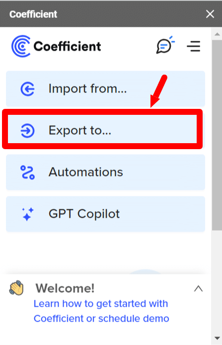
• Step 1: Go to your Google Sheets file, fire up Coefficient, and click ‘Export to…’

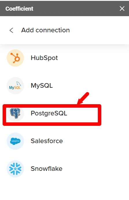
• Step 2: From the list of connectors, choose PostgreSQL.

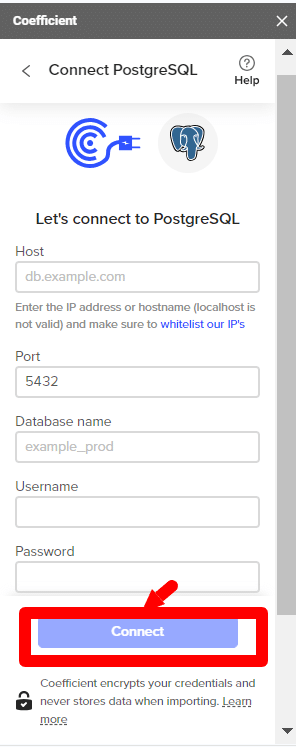
• Step 3: Enter the Postgres database credentials and click on Connect.

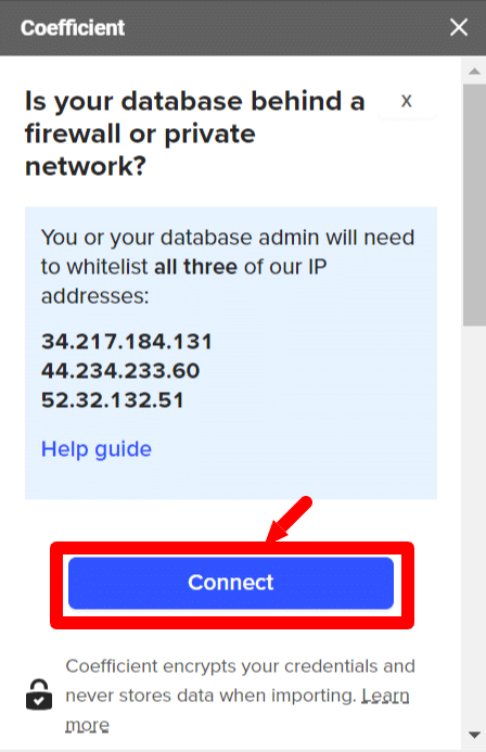
• Step 4: For security reasons, you must whitelist all 3 Coefficient IP addresses to allow data transfer. Click on Connect to do so.

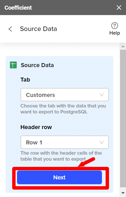
• Step 5: If the connection is successful, you’ll be prompted to enter the tab and header row of the Google Sheets file you want to export to PostgreSQL.

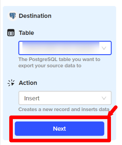
• Step 6: Next, you’ll have to choose the PostgreSQL table to which you want to export your source data and the action you want to take here. You can either choose to update, insert, or delete records from the PostgreSQL table. For our current use case, we want to insert the insert new records into the table:

• Step 7: Match your table columns to the PostgreSQL table columns, and click ‘Save’.
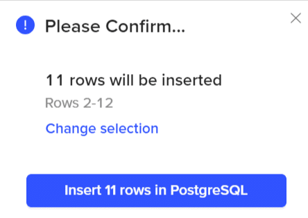
• Step 8: You’ll see a window with all the details about the export.

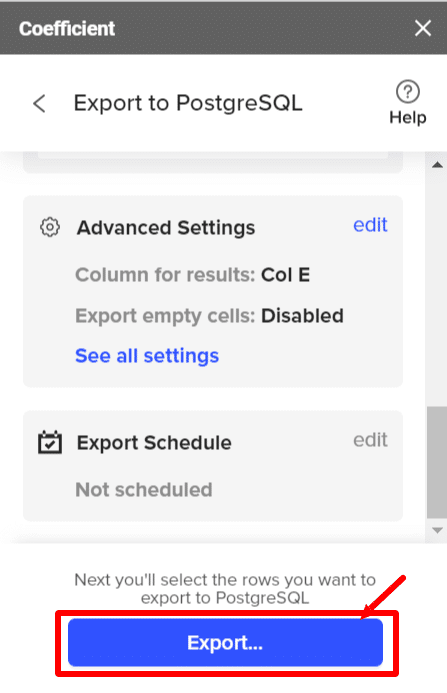
• Step 9: You can choose to export specific rows or all rows on the sheet. For our example, we’ll export all the rows present on the sheet.

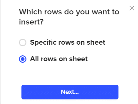
• Step 10: Confirm the selection of your rows. You’ve successfully loaded the transformed and cleaned data into PostgreSQL.

To speed up data retrieval, you can use indexes. 

Create an index on the ‘region’ column:

CREATE INDEX region_index ON customers (c_region);

To list all the indices available on the ‘customers’ table, you can use the \d customers command.

Data Analysis

In this step, we’ll try to look for patterns, identify relationships between variables, and test hypotheses using summary statistics to better understand the data we’ve collected.

Let’s look at a few examples of the types of data analyses we can execute on our data.

Example 1: Calculating the average order value for the south region of the USA.

SELECT AVG (received_amt) AS mean FROM customers WHERE c_region = ‘South’;

You can measure how two variables are related using the statistical correlation measure. The most commonly used correlation measure is the Pearson’s Correlation Coefficient. Pearson’s Correlation Coefficient will give you the following values:

• 0 for no correlation.
  • <0.3-0.5: Low correlation
  • 0.5-0.7: Moderate degree of correlation
  • 0.7-0.9: Strong correlation
  • >0.9: Very strong correlation
• 1 for perfect correlation.
• -1 for perfect negative correlation.

Example 2: Calculating the correlation between regions and customer orders.

SELECT CORR (received_amt, c_region) FROM customers;

Reporting and Visualization

After you’ve analyzed the data, you can simplify the insights obtained through visual representations. With Big Data, it becomes cumbersome to go through thousands of rows and columns in a table/spreadsheet and try to make sense of it. Visual summaries come in handy when trying to identify trends and patterns present in said massive datasets.

Two ways to make dashboards are through spreadsheets and business intelligence tools like Power BI. To make a sales dashboard chart on our data, follow the given steps: 

• Step 1: Choose the columns you’d like to visualize. Click ‘Insert’ -> ‘Chart’ in the Google Sheets menu.
• Step 2: Let’s create a pie chart showing the order distribution by customer region.

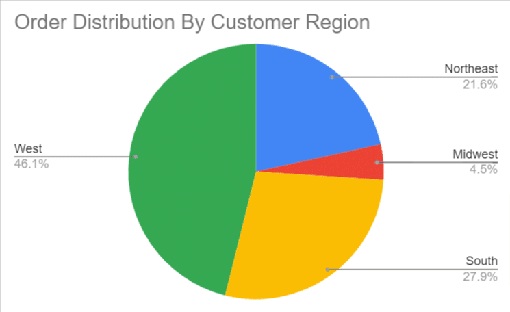
You can customize your chart’s appearance and style, add legends, titles, and texts, and modify the axes, gridlines, and colors accordingly.

The next Postgres data analysis step is to present this to the stakeholders, also known as the data reporting stage. An efficient PostgreSQL reporting tool like Coefficient can provide stakeholders with relevant, accurate, and timely information. 

You could also use Coefficient to trigger email or Slack updates from Google Sheets to inform your team of critical changes or insights.

Data Archiving and Maintenance

Archiving old data is especially important for systems handling large volumes of data. As data ages, it tends to lose relevance for immediate access. 

However, since this data can be helpful in regulatory compliance or historical analysis, you can archive it in a more cost-effective storage solution. This ensures that the primary storage remains responsive and fast.

Note: You can auto-archive your PostgreSQL data by partitioning it.

It is important to have contingency plans in case of a catastrophe like fire, disk failure, or accidentally dropping a critical table, to name a few. An easy solution is to create backup copies of the data regularly. 

You can use the following methods to create PostgreSQL data backups:

• File system-level backup
• SQL Dump
• Continuous archiving

Monitoring database performance is another critical component for application performance since query optimization and resource utilization affect the server’s response to queries. 

This includes keeping track of metrics like logs, active sessions, query performance, replication delay, memory usage, etc.

Automate PSQL Data Imports and Reporting

Coefficient automates PostgreSQL data imports into spreadsheets so that you always work with live data. Its two-way syncing capability automatically bulk exports data from Google Sheets or Excel to PSQL.

Limitations of Doing Data Analysis Using PSQL

PostgreSQL can be handy when executing basic data analyses, but it also has its limitations:

• Pandas performs better than PostgreSQL for large data manipulation, query optimization, and mining operations. PostgreSQL is good for simple data manipulations like data retrieval, filtering, and joins.
• Python and R trump PostgreSQL in data visualization. Python and R provide graphs, charts, and other web-based tools for visualizing data trends, giving users a better idea before jumping into data analysis. Python also lets users analyze visual data through a bunch of easy-to-use tools. 

Summary

PostgreSQL is the go-to option for basic data analysis operations. For more advanced data manipulation, reporting and visualization operations, you might have to opt for other tools/libraries. In this example, we’ve collected, cleaned, and transformed Salesforce data in Google Sheets before exporting it to PostgreSQL for data analysis. Coefficient makes import, export, and visualization of Postgres data incredibly simple, which helps improve efficiency and reduce workload.

Coefficient also allows you to connect 60+ tools to Google Sheets or Excel, allowing you to work with data in a familiar environment, thus reducing the learning curve. Try it for free, and see why Coefficient is the spreadsheet automation tool trusted by over 350,000 professionals worldwide.