Are you tired of constantly scrolling to the top of your Google spreadsheet to check the column headers? If so, you need to learn how to freeze rows in your spreadsheet.
This guide will show you how to freeze rows in Google Sheets, based on examples and step-by-step walkthroughs.
Why Freeze Rows in Google Sheets?
There are many reasons you might want to freeze rows in Google Sheets. Freezing rows in Google Sheets offers a variety of benefits, such as:
1. Keep important data in view. It’s helpful to freeze rows when working with a large, complex spreadsheet, and you want to keep specific rows visible as you scroll. For example, freeze the top row to keep your column names visible or freeze the first few rows to keep your most important data in view.
2. Improve readability. Freezing rows improves your spreadsheet’s readability, especially if you have long rows of data. Keeping certain rows viewable allows you to easily compare data across various rows.
3. Make data entry easier. If you’re working with a team and multiple people enter data into your spreadsheet, freezing rows helps ensure that everyone enters data in the correct location.
The Easiest Way to Freeze a Row in Google Sheets
Freeze a Row with Your Mouse
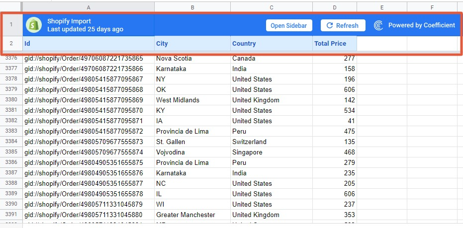
Google Sheets lets you freeze rows in your sheet with a few clicks of your mouse. First, let’s acquire a sample dataset to help illustrate our example. The dataset below was pulled from Shopify into Google Sheets with Coefficient.
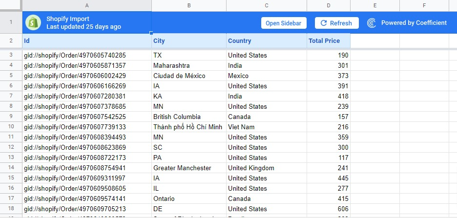
Read our blog post to learn how to connect Shopify to Google Sheets. Now that our data is ready, let’s freeze the top row. Hover your mouse over the empty gray box with two thick gray lines at the top left corner of your sheet.
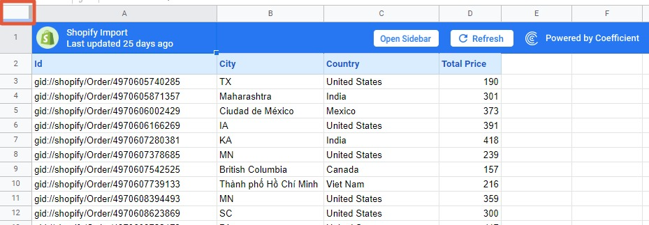
When the hand icon appears, left-click on your mouse and drag the gray horizontal line to the row you want to freeze.
Google Sheets instantly freezes the rows above the gray line, so they stay in view when you scroll down. In our sample table, rows 1 and 2 are still visible, no matter how far you scroll down.
If you want to freeze multiple rows, move the gray line to your desired row. You can’t use this method when freezing a row in the middle of the sheet. You can only use it when freezing rows from the top down.
Use the same method to freeze column A in Google Sheets. Hover your mouse over the same top-left corner cell but this time, select the vertical line and drag it to the right — up to the columns you want to freeze.
Freeze a Row Using the View Menu Option
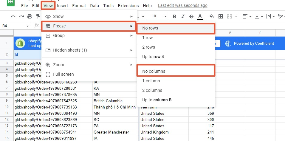
Another way to freeze a row in Google Sheets is through the View option in the top menu. Select the cell where you want to freeze the rows. For instance, select a cell in the second row if you want to freeze the first two rows.
Click on the View tab. Select Freeze -> Up to row 2. If you select a cell in the fourth row, the option will read Up to row 4, and so on.
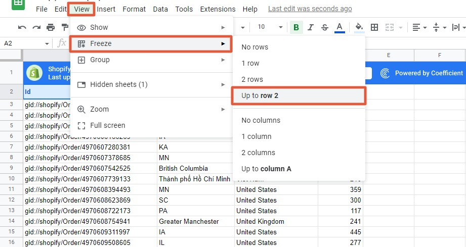
The second and first rows should now be frozen in place. Follow the same method to freeze more than two rows.
Also use the View tab to freeze columns in Google Sheets. Select a cell within the column you want to freeze and click View > Freeze > Up to column B (or up to the column you wish to freeze).

Additionally, you can freeze columns and rows or panes in Google Sheets. A pane consists of Google Sheets rows and columns. To keep your panes in place, freeze the rows and columns using any of the methods above.
Freeze Rows and Columns in the Mobile App
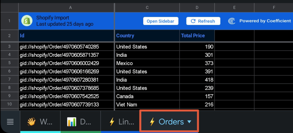
You can freeze cells in the mobile version of the Google Sheets app.
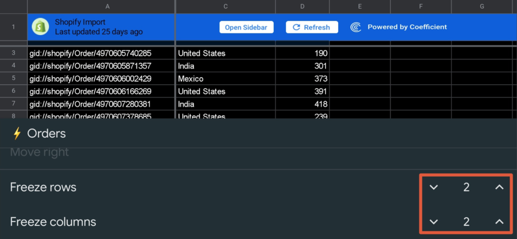
Open your file or sheet on your mobile device and tap on the spreadsheet tab name (Orders in our sample data) to view the options.
Scroll down to the “Freeze rows” and “Freeze columns” options.
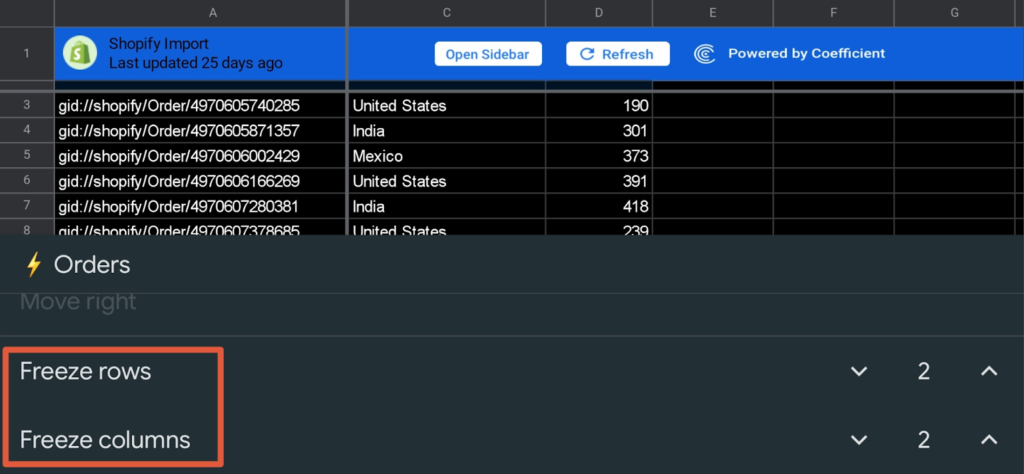
Tap the up and down arrow keys to increase or decrease the number of rows and columns you want to freeze.

Supercharge your spreadsheets with GPT-powered AI tools for building formulas, charts, pivots, SQL and more. Simple prompts for automatic generation.

Tap the back key or outside the window to apply the changes. Your rows and columns will now stick to the top of your spreadsheet.
How to Unfreeze Rows and Columns in Google Sheets
You can unfreeze rows and columns using the two methods below.
First, hover your mouse over the thick line—a vertical gray bar for frozen columns and a horizontal gray line for frozen rows. Left-click and drag up for rows and left for columns to unfreeze them.
The second method is to go back to the View menu tab, select Freeze from the drop-down, and click No Rows or No Columns.
The options unfreeze your rows and columns instantly.
What to Remember When Freezing Rows in Google Sheets
Below are important things to consider when freezing rows in Google Sheets.
- When you freeze rows, Google Sheets creates a new horizontal scroll bar, which you can use to scroll through your frozen rows. You can also use the horizontal scroll bar to scroll the unfrozen rows.
- The frozen rows will remain in the same position regardless of how you sort or filter your data.
- Lock the rows with a password to prevent other users from editing or moving the rows.
- If you change the sheet layout, such as adding or removing columns, the frozen rows may become misaligned. In this case, you need to unfreeze and then re-freeze the rows in the correct position.
- You can freeze multiple rows at once by selecting the number of rows you want to freeze in the “Freeze” option under the “View” menu.
- Freezing too many rows and columns can slow down the sheet if it contains large amounts of data.
Common Issues and Troubleshooting Tips
Below are a few common issues you may encounter when freezing rows in Google Sheets, including possible solutions.
1. Frozen rows do not stay in place. This can happen if you accidentally scroll past the frozen rows. Fix this by clicking the first frozen row to reselect it.
2. Frozen rows are not visible when printing or exporting the sheet. This can be caused by the Print or Export settings. To ensure that the frozen rows are visible when printing or exporting, go to the File menu. Select Print settings or Export settings. Then check the “Include frozen rows option”.
3. Difficulty selecting the rows to freeze. Click the first row you want to freeze and drag the cursor down to select all the rows you want to add as well.
4. Can’t scroll past frozen rows. Fix this by positioning the cursor correctly before scrolling. To scroll past frozen rows, place your cursor just to the right of the frozen rows and scroll up or down.
More “How-To” Google Sheets Articles…
- How to Sort by Date in Google Sheets
- How to Lock Cells in Google Sheets
- How to Add Drop Down List in Google Sheets
- How to Alphabetize in Google Sheets
- How to Wrap Text in Google Sheets
- How to Insert Multiple Rows in Google Sheets
Freeze Rows in Google Sheets to Reference Data Easily
Freezing rows in Google Sheets can improve your spreadsheet data’s readability. It allows you to keep important information visible at all times, making it easier to reference and navigate your most important data.
Additionally, Coefficient’s one-click data connector makes it even easier to sort, analyze, and present reports from your data in Google Sheets.
Get started with Coefficient for free today to pull data from your company systems into Google Sheets effortlessly. Want to get started with a template? Browse through Coefficient’s advanced dashboards and simple spreadsheet templates to find what you need.