How to Add Drop Down List in Google Sheets

The following guide will show you how to add a drop-down list in Google Sheets with ease.

Drop-down lists simplify and streamline repetitive data entry tasks. They make data entry in Google Sheets more accurate and consistent. You can use drop-down lists to avoid typos, misspellings, or other errors. They can also make your data more dynamic in Google Sheets.

This is the ultimate guide to drop-down lists in Google Sheets, based on real examples and step-by-step walkthroughs.

Three Ways to Make a Drop-Down List in Google Sheets

The methods below outline how to add a drop-down list in Google Sheets.

Method 1: Create a Drop-Down List from a Range of Cells

Google Sheets lets you create a drop-down list using an existing dataset in a cell range.

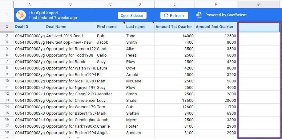
To do this, we’ll need sample data to work with. Let’s use a dataset imported from HubSpot to Google Sheets via Coefficient.

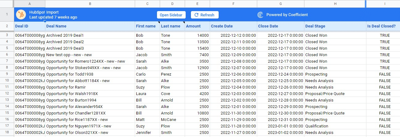
Coefficient is Google Sheets add-on that allows you to pull data from your business systems, such as Salesforce, Looker, HubSpot, and more, into your spreadsheet.

Read this blog post on how to connect HubSpot to Google Sheets for a full walkthrough of the process.

Now that we have our sample dataset, let’s create a drop-down list to enter data for the Deal stage column (column B).

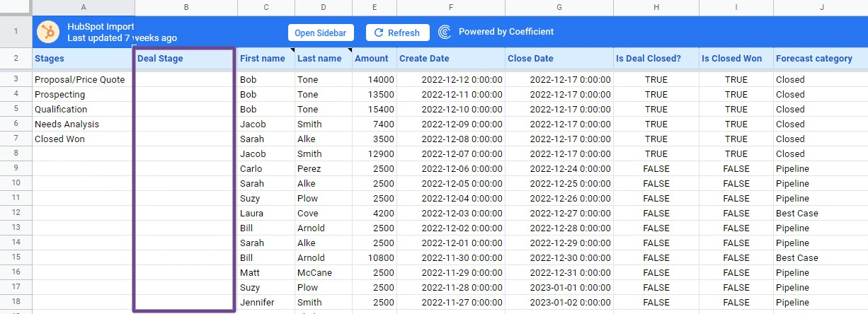
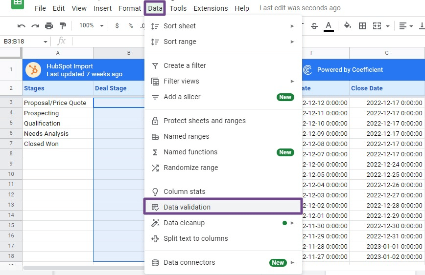
First, select the cell range under column B (B3:B18) and click the Data tab on the top menu. Then click on Data validation.

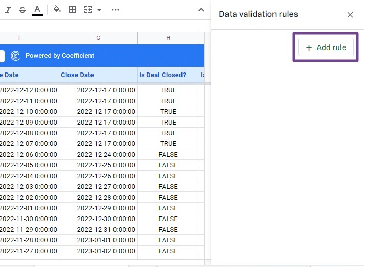
Click on the Add rule button in the Data validation rules side pane.

Ensure you have the correct sheet and range of cells in the Apply to range field. In our example, the range is B3:B18. Then select the Dropdown (from a range) option.

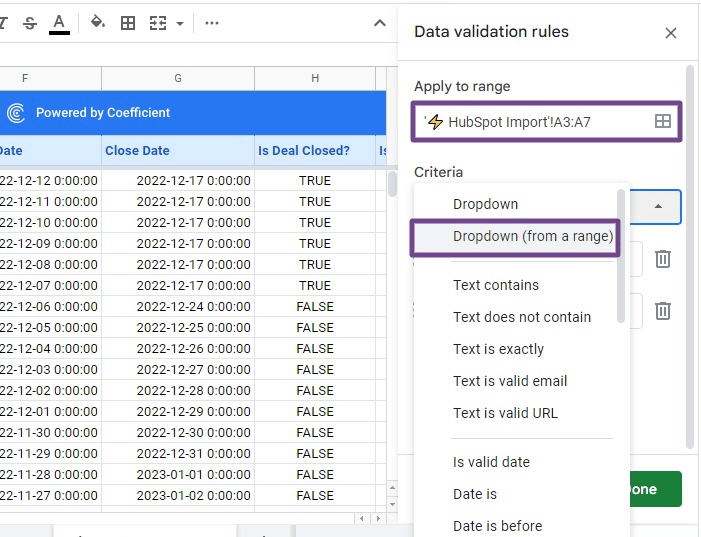
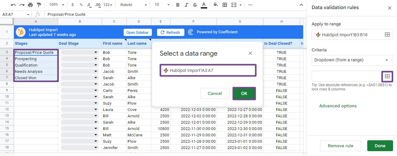
Enter the cell or range address where you want to base your drop-down list (A3:A7).

Google Sheets recommends using absolute references when entering your cell or range address to lock your selected rows and columns.

Your range address with absolute references will look like this:

=$A$3:$A$7

Click the Select a data range icon. Click OK.

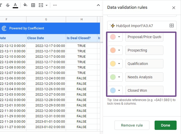
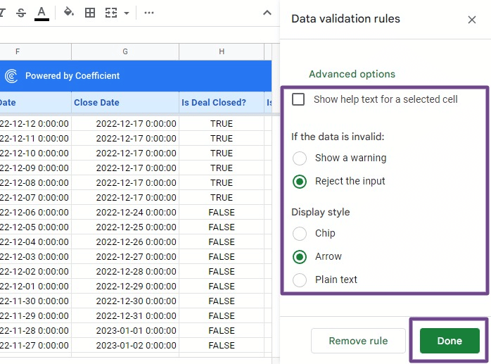
Add custom colors for each drop-down option to make it easy to differentiate the items or values visually.

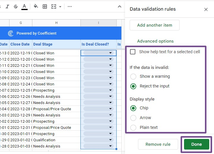
You can also set up advanced options, such as showing help text for selected cells.

Configure specific actions if the data is invalid and choose a display style for your drop-down. Click Done when you’re all set.

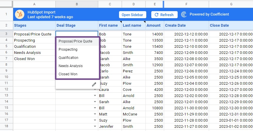
As you can see, you now have the drop-down icons in the column B cells.

Click on the icon at the right corner of each cell. It should show the drop-down’s pre-defined options or values that instantly populate the cell upon selecting them.

The image below shows how the column looks when you fill out your selected cells with your drop-down options.

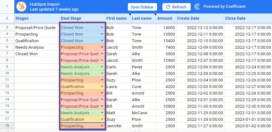
And that’s all there is to it – you’ve just created a drop-down list from a range in Google Sheets.

Method 2: Add a Drop-Down List via Manually Specified Options

You can add a drop-down list in Google Sheets by manually specifying the list’s options instead of creating one from a cell range.

For instance, you could have cells where you want users to input Yes or No or True or False.

Instead of placing these options somewhere in Google Sheets, specify them when creating your drop-down list.

Follow the steps below. We’ll use the same sample dataset from HubSpot.

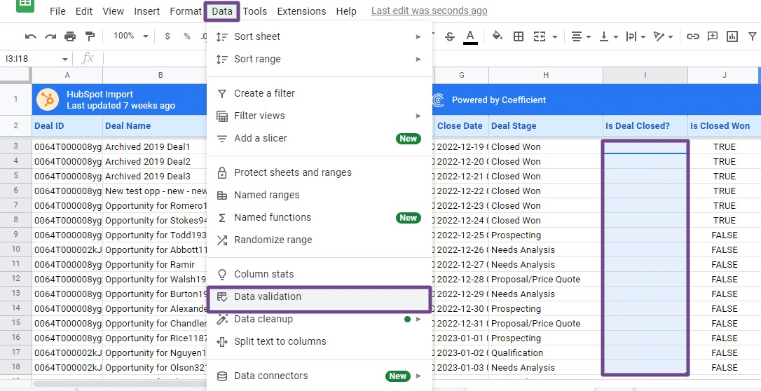
Select the cell range (I3:I18) where you want to apply your drop-down list.

Click the Data option on the Google Sheets menu and select Data validation.

Click Add rule in the Data validation rules side pane. Then select Dropdown as your Criteria.

Type TRUE and FALSE in the option fields and use a custom color for each. Color coding makes distinguishing the data values easy.

You can also apply conditional formatting to color code your drop-down list based on specific conditions. Check out our complete guide to conditional formatting in Google Sheets to learn how.

Include other options if necessary by clicking the Add another item button.

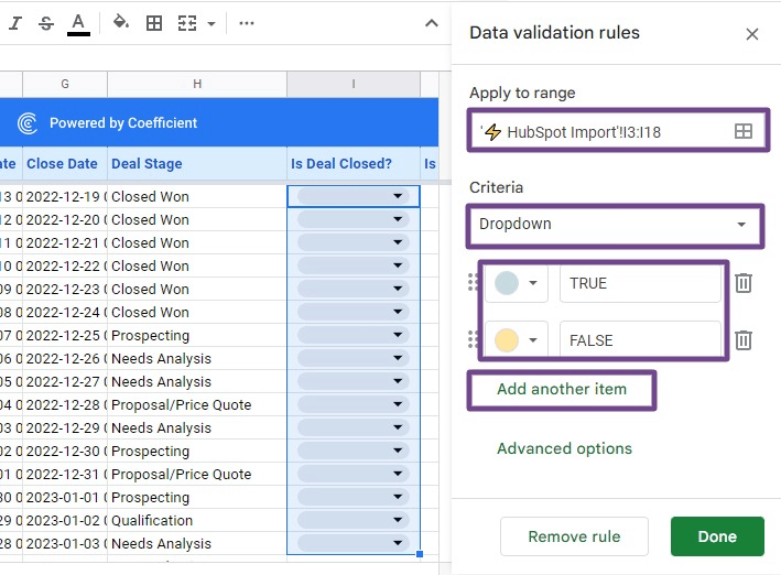
Configure advanced options if you want and click Done.

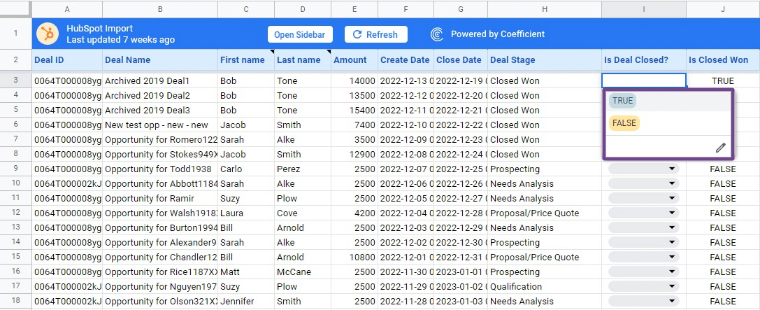
You’ll see the TRUE or FALSE options when you click on the drop-down icon within the cell.

Method 3: Copy an Existing Google Sheets Drop-Down List

You can copy your current drop-down list to another cell, cell range, or multiple cells.

Simply copy cells within the drop-down list, select the range of cells, right-click on your mouse, and click on copy. Another method is to select the cells and use the Ctrl+C keyboard shortcut.

Then paste the cells where you want them in your Google sheet. You can also duplicate the whole column with the drop-down list.

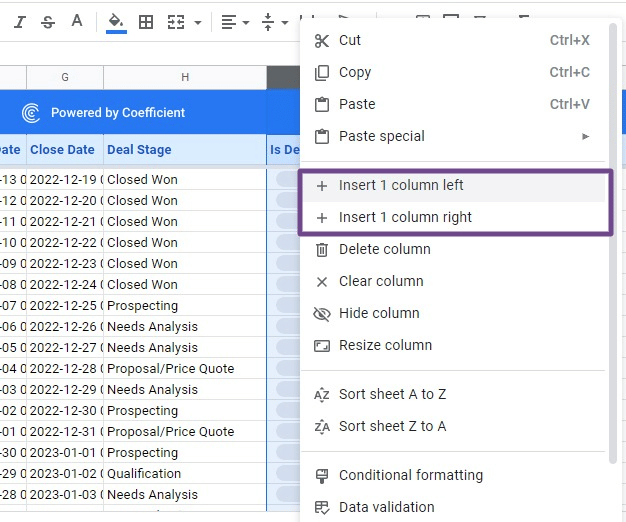
Right-click your mouse on the column header of the cells with the drop-down menu and select Insert 1 column left or Insert 1 column right.

The method allows you to duplicate your existing drop-down lists in Google Sheets quickly.

Duplicating your existing drop-down list this way is best if you want to add the new drop-down menu on either side of the column.

You can copy the drop-down list, excluding its formatting, such as the color code and number format, with the steps below.

• Select the range of cells containing the drop-down list you want to duplicate and copy with your mouse or the keyboard shortcut.
• Right-click your mouse on the cell where you want to place the copied drop-down list.
• Select Paste special and click on Data validation only.

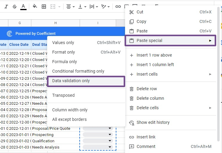
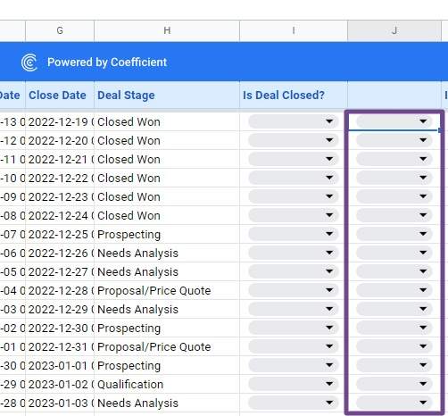
You should see the drop-down list copied to your new column like this:

Adding drop-down lists in Google Sheets is easy with the above methods.

How to Build a Dynamic Chart in Google Sheets using a Drop-Down List

Now that you know how to add drop-down lists in Google Sheets let’s talk about creating dynamic charts with your lists.

Using dynamic charts is a great way to visualize your data without putting everything in one chart or creating several graphs to represent versions or parts of your data.

Dynamic charts make your data visualizations much cleaner, leaner, and less overwhelming.

Let’s create a drop-down list using the same HubSpot data.We’ll add a drop-down list of options to allow another user to control the data view within the chart.

Your drop-down list should let you and other users select a sales representative’s last name, and the chart should display the corresponding data.

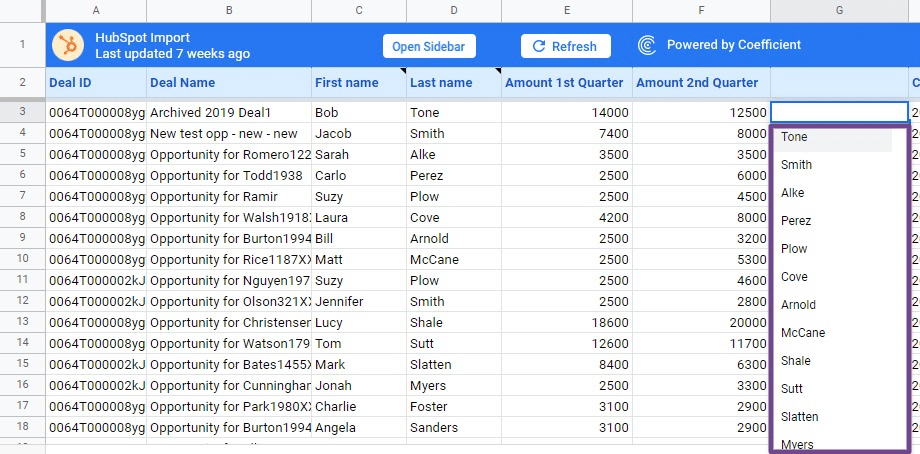
Start by adding a new column in the table (column G in our example).

Next, create a drop-down list from a range of cells. Select G3:G18 and open the Data validation rules side pane as shown in the previous examples.

Add the necessary details and set up your custom drop-down list from the format menu and options accordingly.

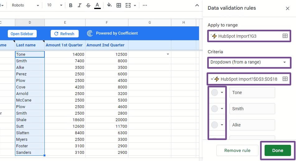
The cell range should be the cell (G3) where you want to apply the drop-down list. Choose Dropdown (from a range) as the Criteria.

Select the range of cells under Last Name (D3:D18) since this is where you base your drop-down list options.

Click Done and Google Sheets should display the drop-down icons in the cells under column G. Click on the icon, and you’ll see the last names as the drop-down list’s options.

Now that we have the drop-down list, let’s use the VLOOKUP Google Sheets formula to retrieve data in a chart dynamically.

If you’re new to using this function, read our ultimate guide to VLOOKUP in Google Sheets.

The aim is to connect your data table to the drop-down list so you can create a data chart corresponding to each name you select.

You can use the VLOOKUP function, which looks for a value and returns the matching result, with your drop-down list to achieve this.

Use VLOOKUP to create a table and pull data from your raw data table via the drop-down list as your search criteria.

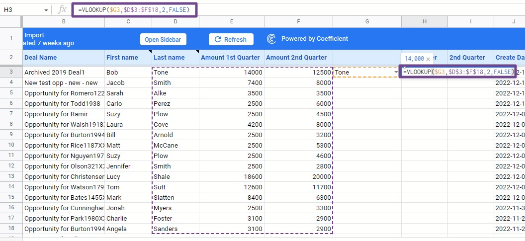
To do this, manually enter or copy and paste this formula in cell H3:

=VLOOKUP($G3,$D$3:$F$18,2,FALSE)

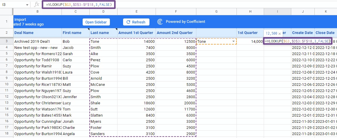
Next, enter the formula below in cell I3:

=VLOOKUP($G3,$D$3:$F$18,3,FALSE)

Finally, you can make a dynamic chart from this data. Select the data range, including the headers (G2:I3), and click Insert on the top menu.

Click on Chart on the drop-down menu to open the Chart editor side pane. Google Sheets automatically creates a suitable chart to represent your data visually.

You can change this by choosing a chart type. For this example, let’s stick to the column chart.

Configure and modify the chart, such as the legend, colors, layout, and other elements under the Setup and Customize options.

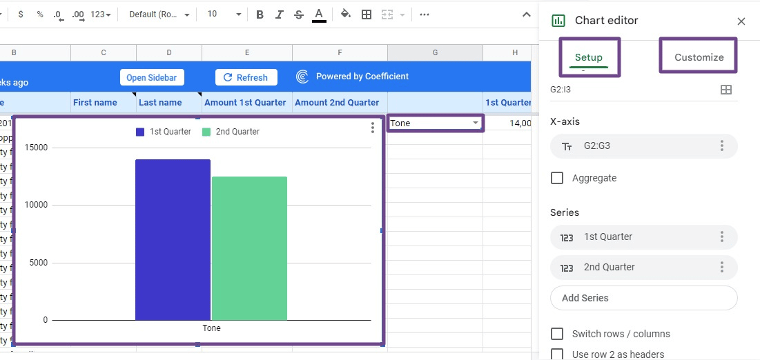
To see another rep’s data, select a different name from your drop-down list in cell G3. You’ll see the corresponding chart based on the drop-down list option you choose.

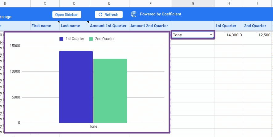
The chart above shows Tone’s first and second-quarter amounts, and the one below shows Perez’s.

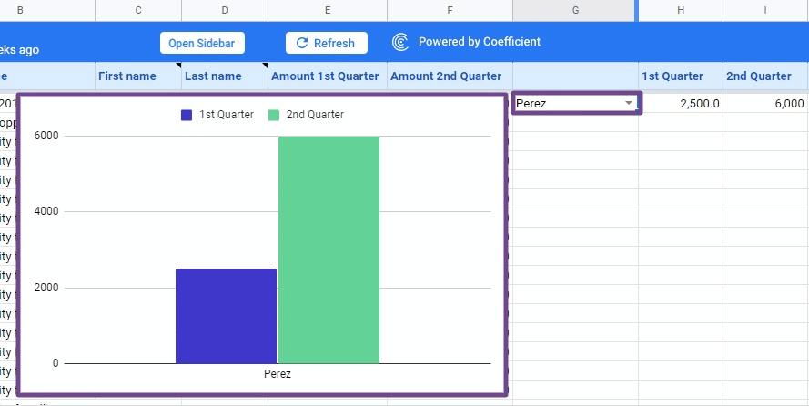
As you can see, your dynamic chart changes to show the corresponding data for each sales rep’s name.

How to Change and Remove a Google Sheets Drop-Down List

Edit your drop-down list in Google Sheets with these steps.

• Open the Data validation rules side pane by clicking on the Data menu option and Data validation.
• Another option is to click on the drop-down (down arrow) icon within the cell and select the Edit button. Both methods open the Data validation rules pane on your screen’s right side.
• Set up the changes you want to make to your drop-down list. You can edit the range of cells where your drop-down list applies, change the color code or remove it, add more items, choose a different display style, and make other modifications.
• You can also add a data validation rule to create another drop-down list within the same Google spreadsheet.
• Click Done, and you’re good to go.

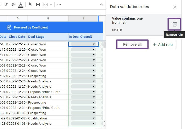
To remove your drop-down list, open the Data validation rules side pane from the Data tab and the Data validation option

You’ll see the side pane with your currently saved drop-down list in the cell and within your spreadsheet.

Click the trash bin icon to remove the data validation rule for your drop-down list individually.

You can also click the Remove all button to delete your existing data validation rules in all the cells.

Manage Your Data in Google Sheets Easily

Use the methods and tools we shared above to create drop-down lists in Google Sheets easily.

By using drop-down lists and spreadsheet templates managing your data in Google Sheets becomes much easier.

Also, remember to use Coefficient so you can simplify the process further. Coefficient syncs real-time business data with Google Sheets, so you can avoid the tedious, time-consuming, and error-prone process of manually copying and pasting data.

Try Coefficient for free now and start pulling data from your business systems in under 60 seconds.