
Select the column or data range you want to alphabetize
Click “Data” in the top menu and select “Sort range” from the dropdown
Choose “Sort range by column (A to Z)” for alphabetical order
For multiple columns, select “Advanced range sorting options” and add additional sort criteria
Click “Sort” and Google Sheets will instantly alphabetize your data
This guide will teach you how to quickly and efficiently alphabetize data in Google Sheets.
Manually sorting spreadsheet data in alphabetical order is time-consuming and tedious. This cumbersome process also leads to misorganization and human error.
However, Google Sheets makes it simple and straightforward to alphabetize data. This guide covers the top methods for alphabetizing data in Google Sheets, through examples and walkthroughs.
Video Walkthrough: How to Alphabetize in Google Sheets
How to Sort Data Alphabetically in Google Sheets
1. Google Sheets Sort Features
Google Sheets offers native sorting tools for alphabetizing your spreadsheet data. Here’s how.
Before we proceed with the example, let’s prepare a sample dataset. We’ll use Coefficient to pull Salesforce data into Google Sheets:
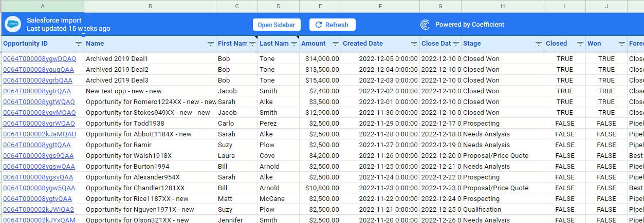
If you want to import live data into Google Sheets, Coefficient is your best option. Coefficient allows you to import real-time data from your business systems, such as Salesforce and HubSpot, into Google Sheets with one click.
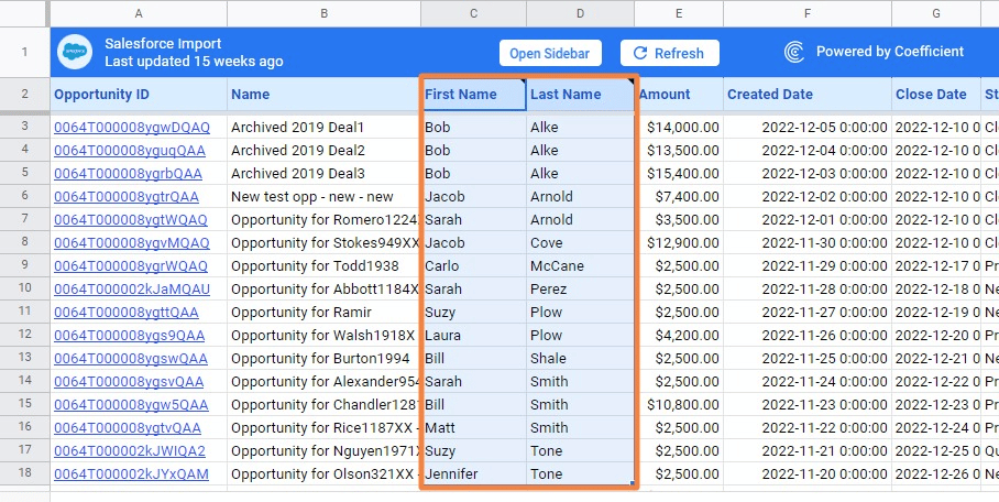
Now that we have our Salesforce dataset, we can start organizing our data alphabetically with the built-in Google Sheets sorting options. Let’s try sorting the Last Name column below in our sample dataset.
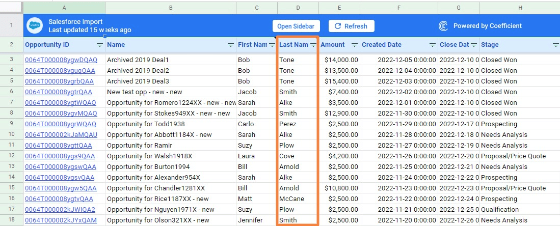
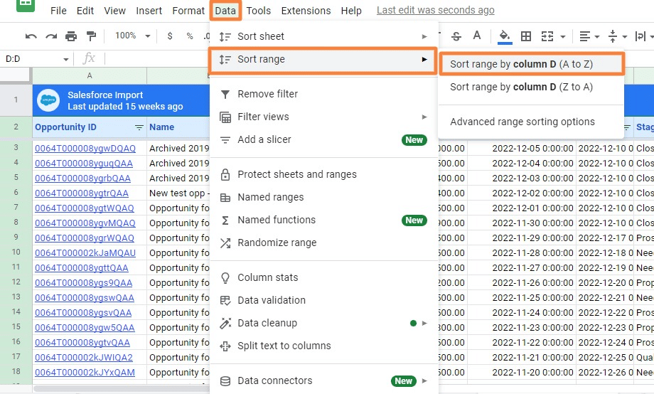
You can sort the last names in the entire column from A to Z by selecting the whole column. Then click Data on the Google Sheets top menu and select Sort range from the drop down menu.
Click Sort range by column D (A to Z).
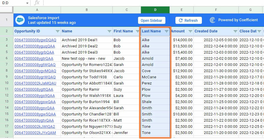
This will sort the column data in alphabetical order.
If you’re alphabetizing data in multiple columns, use the Advanced range sorting options. Select the data range you want to sort.
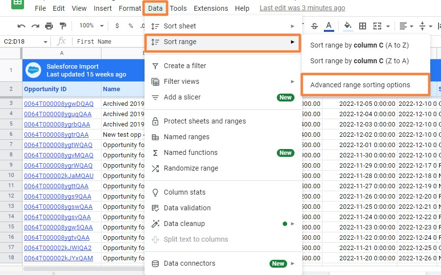
Go back to the Data tab, select Sort range from the drop down menu, then Advanced range sorting options.
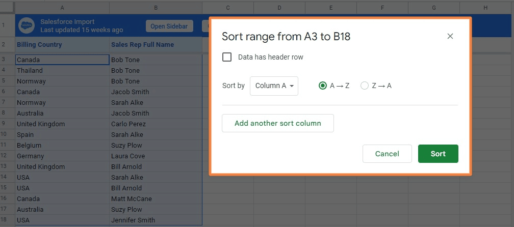
Check the Data has header row box since your column has a header. Click on the Add another sort column button.
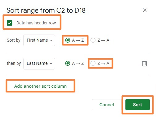
You can also sort your data in reverse alphabetical order (from Z to A).
Select Sort when you’re done. Google Sheets will instantly sort your columns alphabetically.
Alternatively, you can select the data range you want to sort and right-click. Then click on View more cell actions and select Sort range.
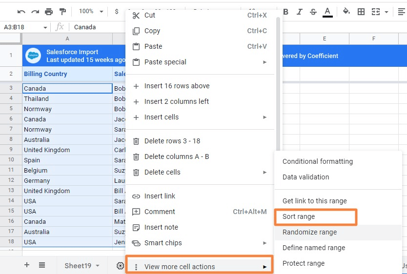
You’ll see the advanced range sorting pop up window, and you can alphabetize your data from there.
Google Sheets lets you undo the alphabetized sorting applied to your data by clicking Undo or Ctrl+Z.
2. Filter Option
The filter option offers another method for alphabetizing data in Google Sheets.
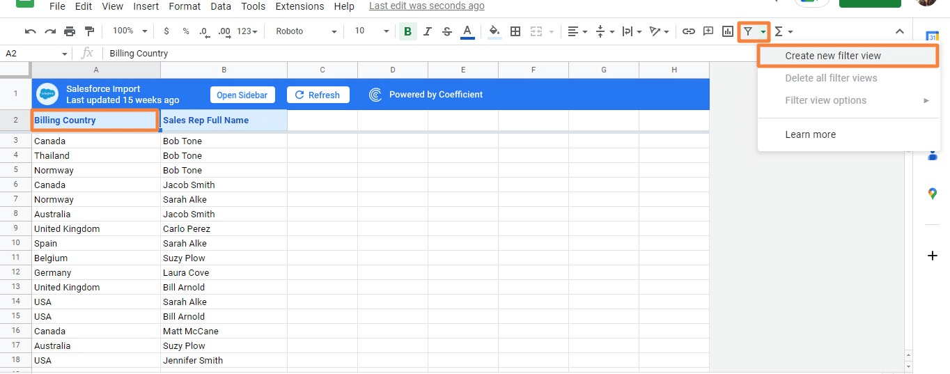
Select the column header of the data you want to sort (cell A2 in our sample dataset below).
Then click on the filter icon in the Google Sheets toolbar. Select Create new filter view from the dropdown menu.
Click on the inverted triangle icon within the header column’s cell. Select the sorting option to alphabetize your data.
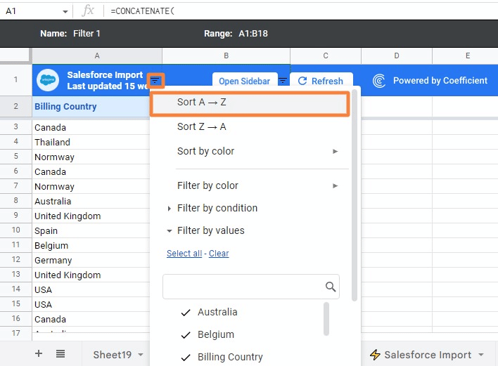
The filter option allows you to sort and filter your column data easily, which helps simplify your data aggregation tasks.
3. SORT Function
In Google Sheets, you can use a SORT function to alphabetize your data.
Let’s start with alphabetizing data in one column. We’ll sort the data under Billing Country (column D) alphabetically.
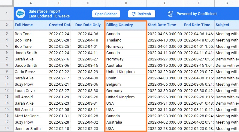
Create a new column on the left side of column D. Enter this SORT formula in cell E3 to alphabetize the data in column D:
=SORT(D3:D18)
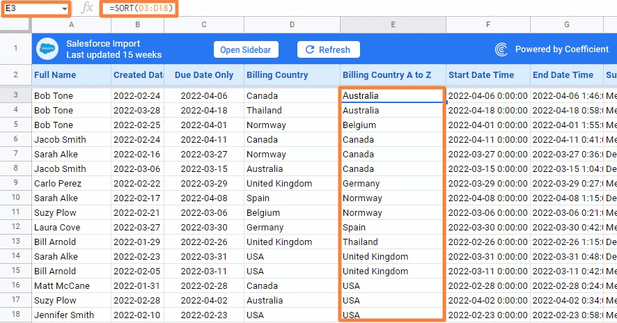
Column E now shows the countries in alphabetical order, with Australia at the top and the USA at the bottom.
Alphabetizing data in Google Sheets with the SORT function provides dynamic data results. If you change the cells, Google Sheets automatically adjusts how the data is sorted, producing an updated result.
However, you can’t sort your data in descending order (Z – A) if you use this formula. You’ll need to include a FALSE argument in your formula to use the SORT function to alphabetize your data in reverse.

Supercharge your spreadsheets with GPT-powered AI tools for building formulas, charts, pivots, SQL and more. Simple prompts for automatic generation.

Let’s do another example, but we’ll alphabetize multiple data columns in Google Sheets this time. Suppose you want to sort the entire dataset below in alphabetical order based on the country names.
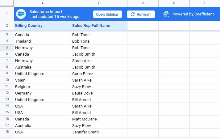
Enter the following formula in a blank cell beside your dataset (cell D3 in this case).
=SORT(A3:B18,1,TRUE)
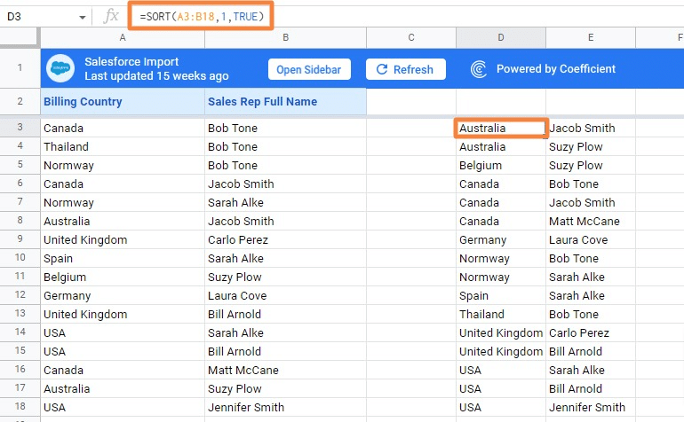
As you can see, both columns are alphabetized based on the Billing Country data column.
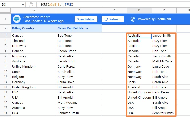
The formula above consists of these three arguments:
- range is the data or cell range you wish to sort.
- sort_column refers to the column’s index in range (or a range outside of range) that contains the values to sort.
- is_ascending can be TRUE to sort your data in ascending order (A to Z) or FALSE to sort in descending order (Z to A).
- sort_column2 , is_ascedning2… are optional arguments referring to the additional columns and sort order flags.
You can alphabetize the dataset from Z to A by replacing the third argument in the formula with FALSE. Your formula will look like this:
=SORT(A3:B18,1,FALSE)
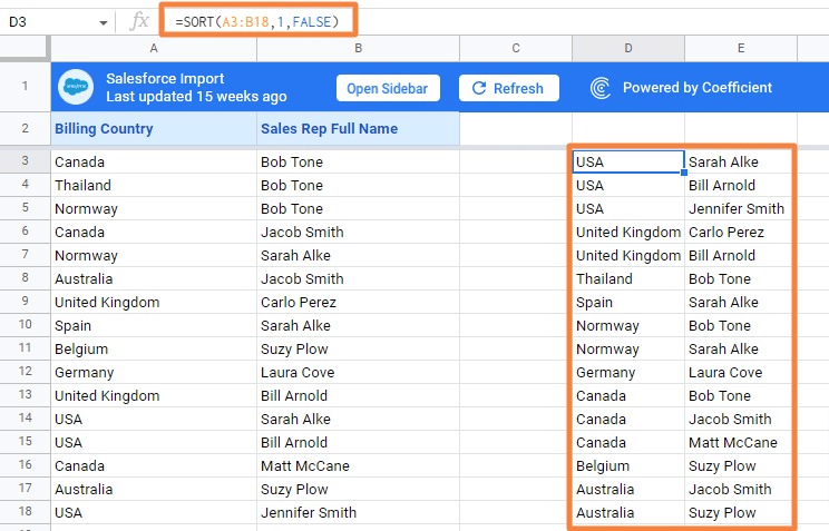
This sorts your dataset in reverse alphabetical order, with the USA at the top, and Australia at the bottom.
4. QUERY Function
You can use the QUERY function to alphabetize data in Google Sheets as well. The QUERY function’s syntax is:
=QUERY(range, “order by sort_column”)
- range is the data or cell range you want to sort.
- sort_column is the column number used for sorting.
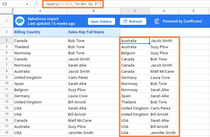
Type the QUERY formula below in a blank cell (C3 in our sample dataset).
=QUERY(A3:B18,”order by A”)
You’ll see your data sorted alphabetically.
Read our blog post on how to use the Google Sheets QUERY function to learn more about using query formulas.
Additional Tip: Freeze Your Header Row
Freezing spreadsheet rows allows you to view data in Google Sheets more easily. The Freeze option locks the rows or columns so they remain on the screen when you scroll down or to the right.
The Freeze option is also helpful when you want to alphabetize data in header rows. This is because, with the Freeze option, your header rows are not sorted with the rest of your data.
You can freeze header rows or columns by selecting the View tab on the Google Sheets menu and then clicking on the Freeze option.
Let’s choose 2 rows as an option since our sample data’s column headers are in the second row.
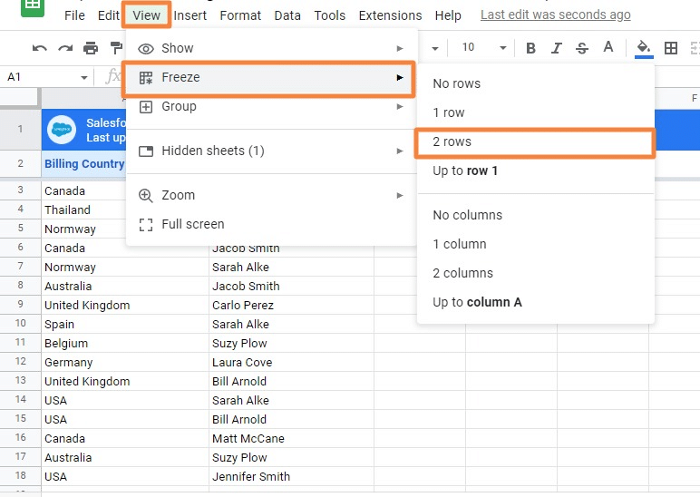
Select the number of columns to freeze.
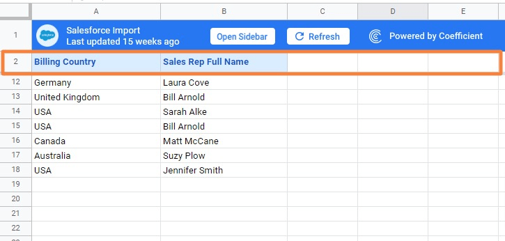
And that’s it! The second row will remain on the screen when you scroll down.
Alphabetize Your Google Sheets Data with Ease
Alphabetizing data in Google Sheets is easy with the right methods, from built-in features, to advanced functions for your specific use case.
And now, with Coefficient, you can sync real-time data from your company systems with Google Sheets, and easily organize it in your spreadsheet.
Try Coefficient for free to streamline data importation into Google Sheets.
