Linking Data Between Multiple Google Sheets: Ultimate Guide

Does linking data between multiple Google Sheets take too much of your time and energy? Need to learn how to link two Google Sheets fast?

Good news. We’re here to share with you several solutions.

We’ll cover several methods that will let you merge your data between multiple Google Sheets so you won’t need to spend a chunk of your time and resources doing this process manually.

By the time you finish going over this guide, you’ll be equipped with a few tried-and-tested techniques to combine your data and Google Sheets seamlessly and efficiently.

Why link data between multiple Google Sheets?

If you don’t link your spreadsheets, you gather and consolidate data from separate files and sheets manually.

Handling data in multiple Google Sheets can take up tons of your time and resources, preventing you and your teams from working with optimum efficiency.

Without linking your multiple spreadsheets, you’ll end up copying and pasting thousands of rows and columns of data, which just won’t cut it.

Also, if your source data changes, you’d have to manually update your datasets and reports by combing through multiple tabs and sheets, which is about as easy as finding a needle in a haystack.

Files like these can be challenging to navigate, and it could take ages before anyone can find the data they’re looking for. Manually processing volumes of data can also lead to errors, causing you to work with inaccurate information.

That is why it’s crucial to link your multiple spreadsheets to help you develop a master view of your consolidated information. This allows you to view and manage your data easily and keeps you from the labor-intensive and time-consuming back and forth process of manually copying and pasting data from various Google Sheets.

TL;DR: Coefficient simplifies and automates linking data between multiple spreadsheets

Coefficient makes linking multiple Google Sheets data a lot easier, more straightforward, let alone, automatic.

With Coefficient, you can choose your Google Sheets data source file, add filters to refine the information you want to pull, and import the data with a few clicks.

Updating your linked spreadsheets is also a breeze since Coefficient lets you configure auto-refresh schedules.

You won’t need to manually update every time your linked source sheet changes or gets new information.

Setting up the data

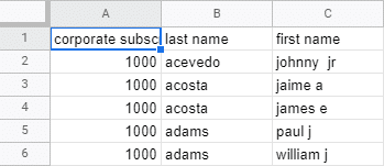
For our example, we’ll use two Google Sheets spreadsheets. We’ll have one spreadsheet named Sales Data that contains two sheets:

• Corporate Subscriptions. This includes a list of companies and their subscription numbers.
• Subscription Details. This contains a list of subscription numbers and their remaining terms and amount still due.

The second one, User Subscriptions, is in an entirely separate spreadsheet. It contains a list of users and their corresponding corporate subscription numbers.

Importing data from another sheet in the same Google Sheets spreadsheet

The steps below outline the ways you can move data from one sheet to another seamlessly. You can also watch our video above for a step-by-step tutorial.

Cell-By-Cell Reference

Using cell-by-cell reference to pull in data from another sheet in the same spreadsheet is pretty straightforward.

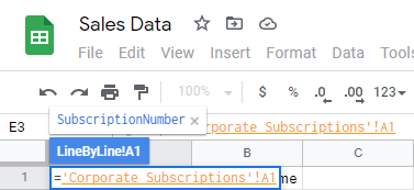
In the first cell where you want the data to appear, type =.

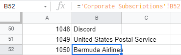
Then, you can either type the name of the sheet enclosed in single quotes, followed by ! and the cell number, like this:

=‘Corporate Subscriptions’!A2

Or, you can click on the sheet, then the cell. You should see the floating formula box that tells you the current formula.

Drag that cell down and to the right to include your desired dataset cells in the row.

While the dataset might look similar to the original data, changes to the data within that range will appear in the sheet that looks up to it.

➔

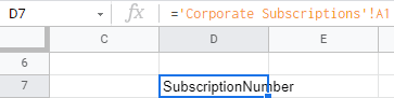
Note: The cell numbers don’t have to match between two sheets. You could import Cell A1 from Corporate Subscriptions into Cell D7 of the working sheet by placing the same formula in D7 instead of A1 like we did in the example:

Range Reference

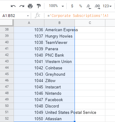
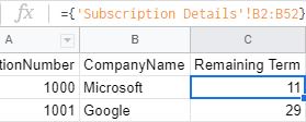
You can pull in an entire column or a specific range without doing all the work in the previous step using this formula:

={‘Subscription Details’!B2:B52}

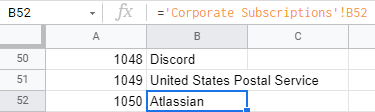
What’s interesting about this approach is that the connection is governed by the cell the formula is entered in, but the other values still update.

vs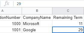 

LOOKUP Function

The LOOKUP function is an invaluable tool for matching up data between two sheets where the data may not be in the same order or is in a one-to-many relationship.

For this to work, you must have a field that you can use as a key (unique to each record you’re looking up) to get perfect results using LOOKUP.

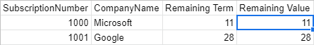
To do this, we’ll go to our Corporate Subscriptions sheet and add a column for Remaining Term and Remaining Value, similar to what we have in the Subscription Details sheet.

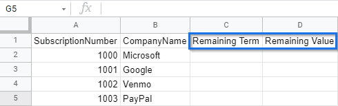
First, click C2, the first cell under our new Remaining Term column, and enter a formula that looks something like this:

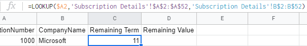
=LOOKUP($A2,‘Subscription Details’!$A$2:$A$52,‘Subscription Details’!B$2:B$52)

The LOOKUP function requires three parts:

• The cell we want to look up (orange)
• The range of cells we expect to find the value in (purple)
• The range of cells that contain the value we want to return (blue)

We’ve used the same syntax previously to select cells in the other sheet, except now we’ve done it with ranges. Specify the $ usage to lock in certain cells.

Also, since we want to find the Remaining Value data and the same SubscriptionNumber, add a $ to lock in that column.

Drag this value down the rest of the cells and all the future rows, so there’s no need to use it on the row number.

Use the $ for the columns and rows of the lookup range (purple) since those won’t change by column or row.

Apply the $ for the row number on the results range (blue) if you don’t want the top and bottom of the range to change. This allows you to get the Remaining Value without rewriting the formula (or any other columns you might have after that).

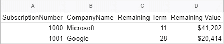
Here’s what we’ve got:

You can drag that formula down and to the right:

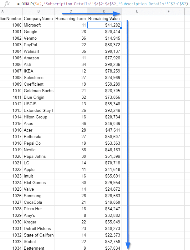
Voila! You’ve joined the data from both those sheets together. Only this time, you can reorder things in the looked-up sheet (Subscription Details) without affecting the data in the Corporate Subscriptions sheet. Updates to data will still reflect, including the data that doesn’t match.

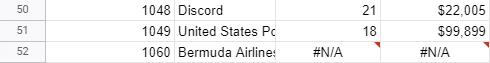
However, the LOOKUP function isn’t perfect. If you change row 52 to subscription 1060 instead of 1050, we still get the result for 1050, because LOOKUP doesn’t give exact matches.

It gives the closest match, which in this case, would be the value for 1050:

 ➔

The benefit of using LOOKUP is that the lookup and the return ranges don’t need to be in the same rows or the same size. The catch is you’re likely only to get an approximated match.

This is where HLOOKUP and VLOOKUP come in handy.

VLOOKUP/HLOOKUP Function

VLOOKUP and HLOOKUP have similar functions, but find values in different ways..

To put it simply, VLOOKUP looks up values within a column (Vertical), and HLOOKUP does the same with values within a row (Horizontal).

Using our original dataset, you can replace the LOOKUP function using this formula:

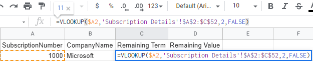
The formula looks a little different from the LOOKUP function.

=VLOOKUP($A2,‘Subscription Details’!$A$2:$C$52,2,FALSE)

The VLOOKUP function requires three parts and includes one optional component:

• The cell we want to look up (orange)
• The full range (including the columns we want to look up), the values we want to return, and everything in between (purple)
• The index of the column we want to return values from, starting with 1 (the lookup column, 2 (the next column to the right), etc.
• (Optional) Google describes this fourth variable as whether the lookup range is sorted. However, Microsoft’s description of this refers to whether you want an approximate match. If you don’t enter this value, VLOOKUP and HLOOKUP will assume the value to be TRUE.

• When TRUE, Google Sheets will assume that your dataset is sorted. If it finds a value greater than your lookup cell, it will return the value just before it. This can mean that if your values are out of order, Google Sheets may return the wrong answers.

• When FALSE, the program will assume that values can be out of order and might encounter a value greater than the lookup value before encountering the lookup value. It needs to keep looking until it finds an exact match, and the cell will return an error if it doesn’t find an exact match.

Specify your $ to lock in your ranges. Lock in the column letter (orange), but leave the row number alone so we can drag it down and to the right and grab the second result.

Lock in the column letters and row numbers of the lookup range, so you know you’re capturing all the data.

You’ll notice that if you’ve copied these values right across, you won’t see any changes.

It’s a quirk to VLOOKUP, and since the function relies on a single range and a column index, you can’t just slide your data over. You’ll need to update your column index.

We entered a 1060 value earlier, and because we require exact matches, VLOOKUP and HLOOKUP show an error (unlike LOOKUP, where we get an approximate value) since it isn’t in the looked-up table.

Video Walkthrough: How to Connect Google Sheets to Google Sheets

Connecting to data in another Google Sheet

Now that you know how to combine multiple spreadsheets into one by linking data within the same sheet, let’s learn to link data between two Google Sheets.

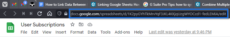
Use the IMPORTRANGE function, which looks like this:

=IMPORTRANGE(“https://docs.google.com/spreadsheets/d/1K2pyGYhTkMrvYqF3JKL4KKjqUzgWYOCcd1-fedLEMiA/edit”,“UserSubscriptions!A1:C10001”)

The formula requires two variables:

• The URL of the spreadsheet you want to pull data from. Copy this from the address bar of the sheet you’re pulling data from and enclose it in quotes.

• The sheet name and range (also enclosed in quotes) using similar syntax we saw back in the Cell-By-Cell reference section. You’ll likely see a reference error, so you’ll need to grant access to the current sheet.

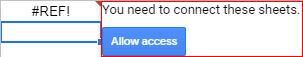
Once you click Allow access (assuming you own both sheets or have edit access to both), the data gets pulled into the sheet:

The changes in the linked sheet eventually get updated (not instantly, but pretty close).

Importing data from another Google Sheet with Coefficient

Let’s go over how Coefficient can help you combine multiple spreadsheets into one using an easier and more streamlined process.

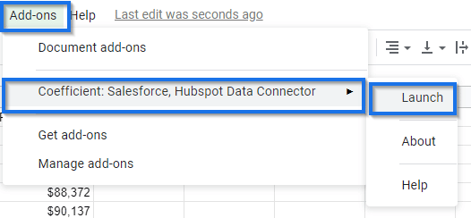
Open the Google Sheets Add-ons menu, click Coefficient: Salesforce, HubSpot Data Connector, then Launch.

Click Import Data on the Coefficient pane.

Then, select Google Sheet.

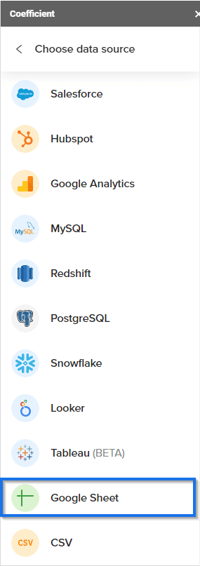
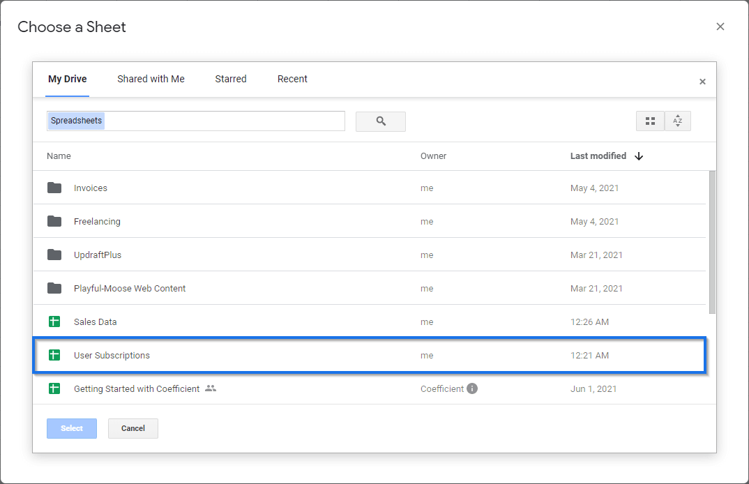
Choose any Google Sheet you want from your Google Drive or other documents you have shared access to.

For this example, let’s pull up the same User Subscriptions list we used in the previous steps and click Select.

Coefficient takes a few seconds to access the data and read the column information. You’ll then see an import panel and the option to filter the data as it comes in.

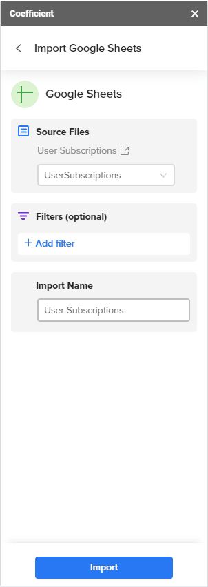
For this example, add a filter for subscription numbers greater than 1025. You could use this to filter out inactive subscriptions or those with more than a certain number of users. Doing this with Coefficient is faster and simpler than the manual process on Google Sheets.

Once you’re done, click Import.

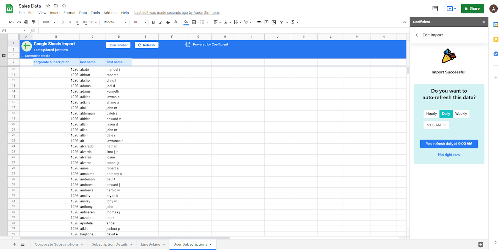
There you have it. Coefficient imports your data almost instantly, and you don’t even need to deal with functions and formulas throughout the entire process.

So maybe now you’re wondering, “How can I get Google Sheets to auto-update a reference to another sheet?”

Coefficient has you covered since it lets you automatically refresh that data on a schedule, so you won’t need to do it painstakingly and manually.

The IMPORTRANGE solution allows you to import entire columns at once, but you’ll need to specify bounds for it or it will disrupt your dataset if your data moves too much.

Also, IMPORTRANGE doesn’t offer a built-in way to filter data, so you’ll need to do this separately.

Coefficient takes care of both problems for you by building the filter into the import, including importing any populated rows or columns seamlessly.

Another benefit to using Coefficient is when you want to generate reports for your presentations and don’t want your data to be updated in real-time.

Your data gets automatically updated when you use the IMPORTRANGE function, and it happens as soon as the source spreadsheet data is changed.

This means that if you’re preparing a presentation from a live document, you would need to either create a copy or the owner needs to stop updating the file while you finish your task.

You can already guess the confusion and disruption that can happen when many people work on the same document at the same time.

However, Coefficient can sync on demand, saving you from these challenges. You can do a final sync and then prepare your presentation materials without the source data changing or the linked tables getting rewritten and blowing up your spreadsheet in the process.

Conclusion

The methods introduced in this guide helps you streamline the process of linking spreadsheet data between multiple Google Sheets.

As you link multiple Google Sheets together, allowing the files to interact with each other automatically, you can increase your productivity and the accuracy of your data.

With the amount of stress, frustration, and manpower expense you’ll shave off by automating the process of linking Google spreadsheets, you can focus on running your business better.

Try Coefficient for free today!