How to Use the Excel FILTER Function: A Step-by-Step Tutorial

The Excel FILTER function sorts data based on specific criteria. Learn to apply this versatile tool for efficient data management and analysis in spreadsheets.

Using the Excel FILTER Function: Step-by-Step Guide

Applying a Simple Filter

The FILTER function allows you to extract data that meets certain conditions. Here’s how to use it:

Step 1. Select the data range you want to filter.

• Open your Excel spreadsheet and identify the range of cells containing your data.
• Note the column letters and row numbers of your data range.

Step 2. Enter the FILTER function syntax.

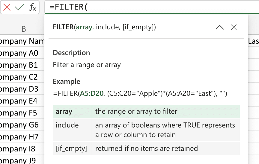
• In a blank cell, type =FILTER(
• The basic syntax is: =FILTER(array, include, [if_empty])

Step 3. Specify the criteria for filtering.

• For the array argument, enter the range of cells you want to filter.
• For the include argument, define your filter condition.
• Optionally, add an [if_empty] argument to specify what to display if no results match.

Step 4. Press Enter to see the filtered results.

• Excel will display only the rows that meet your specified criteria.
• The results will automatically update if your source data changes.

Step 5. Adjust the formula as needed for dynamic filtering.

• Replace hard-coded values with cell references to create flexible filters.
• Use logical operators to combine multiple conditions.

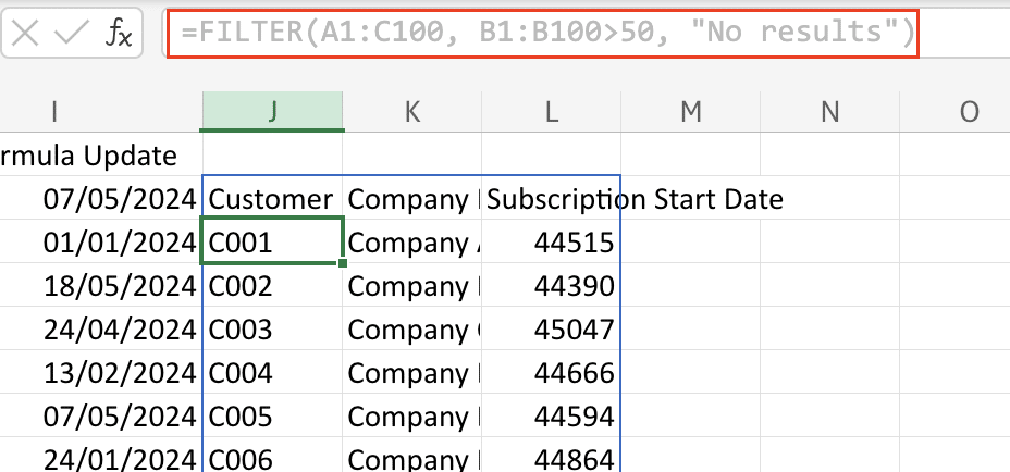
Example: =FILTER(A1:C100, B1:B100>50, “No results”)

This formula filters rows where column B values are greater than 50, displaying “No results” if nothing matches.

Filtering with Multiple Criteria

To filter data based on multiple conditions:

Step 1. Use the same FILTER function syntax.

• Start with =FILTER( as before.

Step 2. Combine multiple conditions using logical operators.

• Use * for AND operations, + for OR operations.
• Enclose each condition in parentheses for clarity.

Example: =FILTER(A1:C100, (B1:B100>50) * (C1:C100=”Complete”))

This filters rows where column B is greater than 50 AND column C is “Complete”.

Step 3. Nest conditions for complex filtering.

• Use parentheses to group conditions and control the order of operations.

Example: =FILTER(A1:D100, ((B1:B100>50) + (C1:C100=”High”)) * (D1:D100<>”Cancelled”))

This filters rows where (B>50 OR C=”High”) AND D is not “Cancelled”.

Step 4. Use wildcard characters for text-based filtering.

• Use * to represent any number of characters, and ? for a single character.

Example: =FILTER(A1:C100, ISNUMBER(SEARCH(“New*”, B1:B100)))

This filters rows where column B starts with “New”.

Filtering Multiple Columns

To filter and return data from multiple columns:

Step 1. Expand the array argument to include all desired columns.

• Instead of A1:A100, use A1:D100 to include columns A through D.

Step 2. Use structured references for table data.

• If your data is in an Excel table, use table references for cleaner formulas.

Example: =FILTER(Table1, Table1[Status]=”Active”)

This filters all columns in Table1 where the Status column is “Active”.

Step 3. Return specific columns from a larger dataset.

• Use the CHOOSE function to select specific columns to return.

Example: =FILTER(CHOOSE({1,2,4}, A1:A100, B1:B100, D1:D100), C1:C100>1000)

This filters columns A, B, and D based on values in column C.

Step 4. Handle blank cells in the filtered results.

• Use the IFNA function to replace #N/A errors with blank cells or custom text.

Example: =IFNA(FILTER(A1:C100, B1:B100>50), “No matching data”)

This displays “No matching data” instead of #N/A when no results are found.

Creating Dynamic Filters with Cell References

To create flexible, user-friendly filters:

Step 1. Replace hard-coded criteria with cell references.

• Instead of B1:B100>50, use B1:B100>$E$1, where E1 contains the threshold value.

Step 2. Use named ranges for easier formula management.

• Define names for your data ranges and criteria cells.
• Use these names in your FILTER formulas for improved readability.

Step 3. Create a user-friendly filter interface.

• Set up cells for users to input filter criteria.
• Use data validation to create dropdown lists for selecting filter options.

Step 4. Update filtered results automatically.

• Excel recalculates FILTER functions automatically when source data or criteria change.

Step 5. Combine FILTER with other functions like SORT or UNIQUE.

• Nest FILTER within other functions to further process your filtered data.

Example: =SORT(FILTER(DataRange, CriteriaRange=FilterCriteria), 2, 1)

This filters data based on user-selected criteria, then sorts the results by the second column in ascending order.

Understanding the Excel FILTER Function

What is the FILTER Function?

The FILTER function in Excel extracts rows from a range or array that meet specified conditions. It offers several advantages:

1. Dynamic results: Filtered data updates automatically when source data changes.
2. Multiple criteria: Apply complex filtering conditions easily.
3. Array output: Returns multiple rows and columns without array formulas.
4. Performance: Generally faster than AutoFilter for large datasets.

FILTER is available in Excel 365 and Excel 2021. For older versions, consider using INDEX and MATCH or Advanced Filter as alternatives.

When working with large datasets (100,000+ rows), FILTER may slow down spreadsheet performance. In such cases, consider using Power Query or database connections for data manipulation.

FILTER Function Syntax and Arguments

The FILTER function uses the following syntax:

=FILTER(array, include, [if_empty])

Let’s break down each argument:

1. array: The range of cells or array to filter.
   • Can be a single column or multiple columns.
   • Example: A1:C100 or Table1

1. include: A logical test that determines which rows to keep.
   • Must result in TRUE/FALSE for each row in the array.
   • Can use comparison operators (=, >, <, etc.) and logical functions (AND, OR, NOT).
   • Example: B1:B100>50 or ISNUMBER(C1:C100)

1. [if_empty] (optional): What to return if no rows meet the criteria.
   • If omitted, FILTER returns #CALC! when no rows match.
   • Can be text, a number, or a cell reference.
   • Example: “No matches found” or 0

Common errors to avoid:

• #CALC!: No rows meet the filter criteria (add an [if_empty] argument to handle this).
• #VALUE!: The include argument doesn’t result in a boolean array.
• #SPILL!: Not enough empty cells to display the result (ensure sufficient space below the formula).

You can nest FILTER within other functions, but be cautious of circular references:

Example: =AVERAGEIF(FILTER(A1:B100, A1:A100>0), “>10”)

This calculates the average of values greater than 10 from a filtered range where column A is positive.

Advanced Applications of the Excel FILTER Function

Combining FILTER with Other Excel Functions

FILTER becomes even more powerful when combined with other Excel functions:

1. FILTER with SUMPRODUCT for conditional sums:

=SUMPRODUCT(FILTER(B1:B100, A1:A100=”Category1″))

This sums values in column B where the corresponding value in column A is “Category1”.

2. Creating dynamic charts using FILTER:

1. Create a FILTER formula to extract relevant data.
2. Name the range containing the FILTER formula.
3. Use this named range as the source for your chart.

The chart will update automatically when the filtered data changes.

3. FILTER in array formulas:

=SUM(FILTER(B1:B100, A1:A100=”Category1″) * FILTER(C1:C100, A1:A100=”Category1″))

This multiplies corresponding values from two filtered columns before summing the results.

4. Complex data analysis example:

=AVERAGE(FILTER(C1:C100, (A1:A100=”Category1″) * (B1:B100>QUARTILE(B1:B100, 3))))

This calculates the average of values in column C where A is “Category1” and B is in the top quartile.

Limitations and workarounds:

• FILTER can’t directly reference its own output (to avoid circular references).
• For complex, multi-step filtering, consider using multiple FILTER functions or combining with LET for intermediate calculations.

How to Filter in Excel with Multiple Criteria?

Let’s explore more advanced multiple criteria filtering:

1. Filtering based on date ranges:

=FILTER(A1:C100, (B1:B100>=DATE(2024,1,1)) * (B1:B100<=DATE(2024,12,31)))

This filters rows where column B dates fall within the year 2024.

2. Filtering with partial text matches:

=FILTER(A1:C100, ISNUMBER(SEARCH(“product”, A1:A100)))

This keeps rows where column A contains the word “product” (case-insensitive).

3. Filtering based on calculated results:

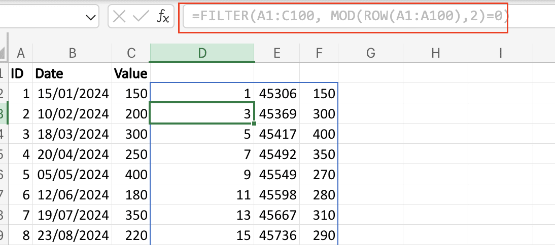
=FILTER(A1:C100, MOD(ROW(A1:A100),2)=0)

This filters to keep only even-numbered rows.

4. Optimizing complex filters:

• Use helper columns for complex calculations to simplify FILTER formulas.
• Combine multiple FILTER functions with CHOOSE for intricate logic.
• Consider using LET function (if available) to create named sub-expressions for cleaner formulas.

Example of a complex filter using LET:

=LET( data, A1:D100, dates, INDEX(data,,2), values, INDEX(data,,3), categories, INDEX(data,,4), FILTER(data, (dates>=TODAY()-30) * (values>AVERAGE(values)) * (categories=”High Priority”) ) )

This filters rows from the last 30 days with above-average values and “High Priority” category.

Wrap-up

The Excel FILTER function is a versatile tool for data analysis and reporting. Practice with different criteria and combinations to fully leverage its capabilities in your spreadsheets. Experiment with the examples provided to enhance your Excel skills and streamline your data management tasks.

Ready to take your Excel data analysis to the next level? Try Coefficient to seamlessly integrate live data from various business systems directly into your spreadsheets. Get started with Coefficient today and revolutionize your data workflow.