The Ultimate Guide to VLOOKUP in Google Sheets

If you’re working with volumes of interrelated data in spreadsheets, finding and referencing information across tables is often challenging. That’s where VLOOKUP comes in. VLOOKUP is a powerful, but sometimes overlooked, function in Google Sheets that retrieves matching data between two distinct tables. 

When used properly, VLOOKUP can decomplexify spreadsheet processes and speed up data analysis. In this guide, we’ll cover the nuts and bolts of VLOOKUP, including how to use it in Google Sheets.

What is VLOOKUP in Google Sheets?

VLOOKUP is a search function that finds data in one table and uses this data within another table. The tables can occupy the same sheet, a different tab, a separate sheet, or a spreadsheet file. The function searches a specified column vertically for a search key (hence VLOOKUP), then returns the value from the same row. 

Google Sheets VLOOKUP: Syntax & Function

Let’s break down the basics of a VLOOKUP formula to better understand how it works. Here’s an overview of the standard syntax:  

VLOOKUP(search_key, range, index, [is_sorted])

• index is the column containing the value you’re looking for. For instance, if you want to find the product price in a table, this would be the price column. The index value should be between 1 (first column) and the total number of columns.
• search_key is the item or value you want to find. For instance, if you’re looking for a product in your inventory table, the search_key could be the item number or product name in the same row. 
• range refers to the range you want to include in the VLOOKUP function or the data columns.
• is_sorted refers to the final value and is true or false (true by default). It is used to indicate whether the index column has been sorted.  

VLOOKUP in Google Sheets: Key Points

While VLOOKUP is a powerful function, it’s not without limitations. Consider these factors before using VLOOKUP to avoid potential errors.  

• VLOOKUP is not case sensitive. The function does not distinguish between uppercase and lowercase letters. 
• VLOOKUP does not search columns to the left of the specified range. To search columns to the left, you must use an Index Match formula. 
• When is_sorted is set to TRUE, you must sort the range’s first column in ascending order. 
• VLOOKUP can search using partial matches based on wildcard characters: the asterisk (*) and question mark (?).
• Set the is_sorted to FALSE to return exact matches. For instance, if your VLOOKUP from another sheet returns incorrect results.  

How to use VLOOKUP in Google Sheets 

Video Tutorial: How to Use VLOOKUP in Google Sheets

Now that you understand the function better, let’s actually get into the nuts-and-bolts of using VLOOKUP. Here are several ways you can use VLOOKUP in Google Sheets. Also, see our video tutorial above for a full walkthrough on how to use VLOOKUP.  

1. VLOOKUP within the Same Google Sheet

Let’s say you have a Sheet containing your product IDs, a pricing schema, prices, and subscriptions for your SaaS products. 

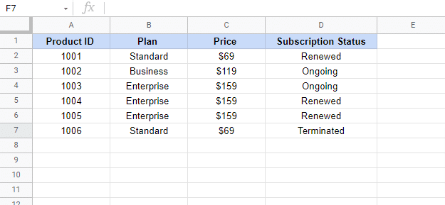
You want to produce another table within the same Sheet that only includes the product ID and price. To do this, you can use VLOOKUP to extract the price from the spreadsheet using only the product ID number. Here’s how. 

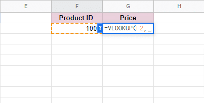
Step 1: Create another column for the Product ID and Price. 

Input the product ID number you want to find, then in the field right next to it under the Price column, type in =VLOOKUP, and enter the formula’s parameters.  

Step 2: Input the search key 

Enter the product ID value into the formula or click the cell (F2) to automatically add it. Then add a comma.

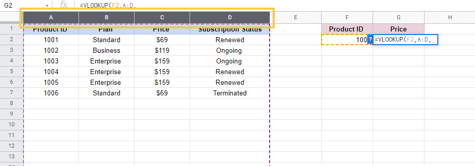
Step 3: Add the range (second parameter) and specify the set of columns you want to include in the search. 

Click the first column header and drag your mouse to the table’s last column, or type in A:D, then type a comma.   

Step 4: Input the column containing the value you’re looking for

Enter the number of the column that contains the value you’re looking for. The price is the third column in the sequence, so type ‘3’. Then add a comma after. 

Step 5: Enter ‘False’ for is_sorted

Add False after the last comma and include a closing parenthesis. 

Your final formula should look like this:

=VLOOKUP(F2,A:D,3,FALSE)

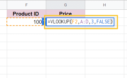
Step 6: Execute VLOOKUP formula

Press Enter, and you should see the result appear in the cell with the VLOOKUP formula. 

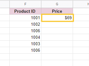
Step 7: Drag down VLOOKUP formula

Drag the cell down to copy the formula to the rest of the cells in the column. 

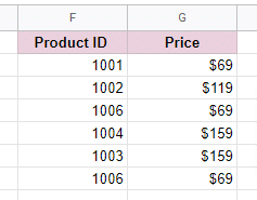
You’ll get the data you need quickly without manually looking up each corresponding value and inputting them to the new table. 

AI + Google Sheets: Use Formula Builder to Automatically Generate VLOOKUP Formulas

You can also use Coefficient’s free Formula Builder to automatically create the formulas in this first example. To use Formula Builder, you need to install Coefficient. The install process takes less than a minute.

We’ll outline how to install Coefficient from the Google Workspace Marketplace. Or you can skip the marketplace altogether, and get started for free right from our website. 

First, click Extensions from the Google Sheets menu. Choose Add-ons -> Get add-ons. This will display the Google Workspace Marketplace. Here a direct link to Coefficient’s Google Workspace Marketplace listing. 

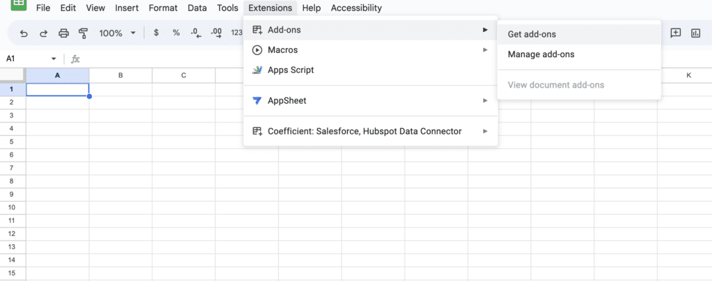
Search for “Coefficient”. Click on the Coefficient app in the search results.

Accept the prompts to install. Once the installation is finished, return to Extensions on the Google Sheets menu. Coefficient will be available as an add-on.

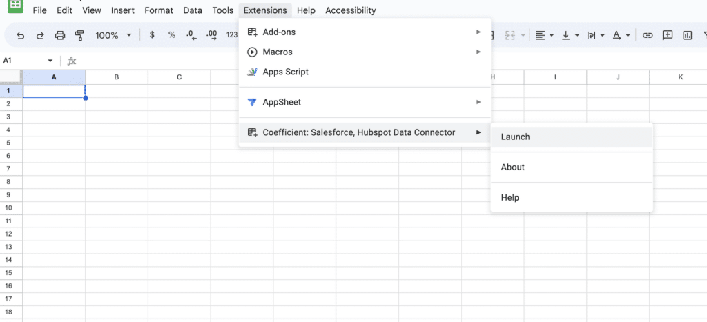
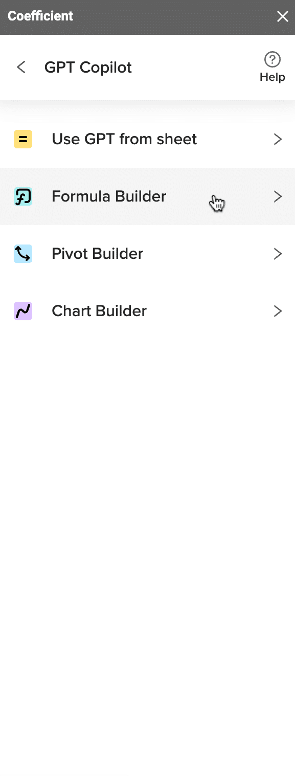
Now launch the app. Coefficient will run on the sidebar of your Google Sheet. Select GPT Copilot on the Coefficient sidebar.

Then click Formula Builder.

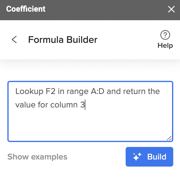
Type a description of a formula into the text box. For this example, type: Lookup F2 in range A:D and return the value for column 3.

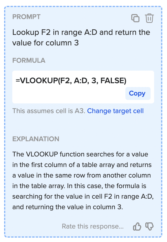
Then press ‘Build’. Formula Builder will automatically generate the formula from the first example.

2. VLOOKUP with Wildcard Characters

If you only know part of a search_key, perform VLOOKUP for partial matches using these wildcard characters:

• A question mark (?) to match single characters
• An asterisk (*) to match character sequences

Let’s say you want to retrieve information about a specific product from the same table.

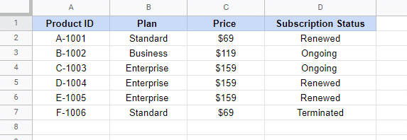
If you don’t know the entire product ID, but remember the first character “A,” use an asterisk to fill in the missing part in your formula:

=VLOOKUP(“A*”,A:D,1,FALSE) 

Press Enter and see the output: 

Create a more flexible VLOOKUP formula by entering the known part of the search key in a cell. Then string that cell with ‘*’. Next, set the is_sorted perimeter to TRUE.   

For instance, you can pull the corresponding pricing plan using this formula:

=VLOOKUP($F$1&”*”,A:D,2,True) 

To pull the actual price, use this formula: 

=VLOOKUP($F$1&”*”,A:D,3,True) 

3. Case-Sensitive VLOOKUP

As mentioned, VLOOKUP does not distinguish between lower and uppercase letters.

If you need to do a case-sensitive lookup, use INDEX MATCH with the EXACT and TRUE functions in your Google Sheets VLOOKUP array formula: 

ArrayFormula(INDEX(return_range, MATCH (TRUE,EXACT(lookup_range, search_key),0)))

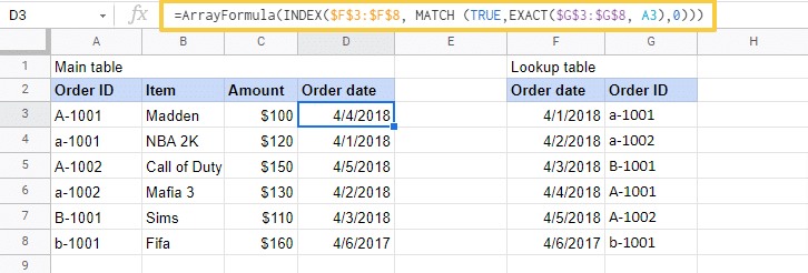
Using the sample table below, let’s assume that the search key is in cell A3, the lookup range is G3:G8, and the return range in F3:F8. 

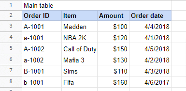
The formula should look like this:

=ArrayFormula(INDEX($F$3:$F$8, MATCH (TRUE,EXACT($G$3:$G$8, A3),0))) 

The formula can distinguish between lowercase and uppercase characters (a-1001 and A-1001). 

4. VLOOKUP on another Sheet within the Same Spreadsheet File

Suppose you have an ‘Employees’ table in one Sheet, and a ‘Sales’ table in another Sheet. 

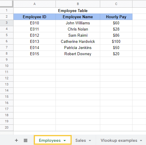
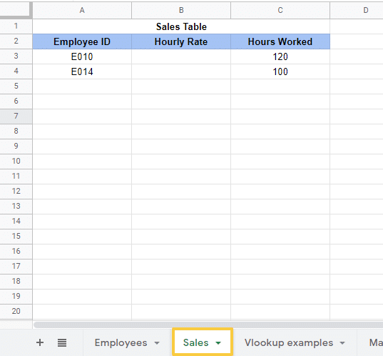
Here’s how to retrieve the Hourly Rates that correspond to Employee IDs E010 and E040 from the Employees Sheet, and display them in cells B3 and B4 of your Sales sheet. 

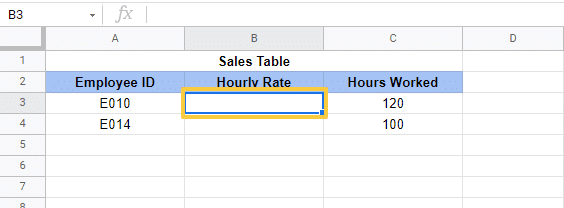
Step 1: Select target cell

Click on your target column’s first cell (cell B3 in the Sales Sheet).  

Step 2: Define the search key

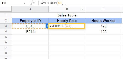
Input this:

=VLOOKUP(A3, 

A3 is the cell that contains the value you want to look up. 

Step 3: Set the search range to specific columns on the other Sheet

Input the search range by clicking and opening the Employees tab. 

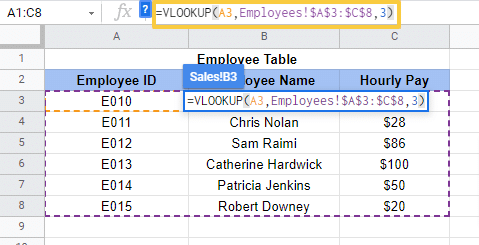
Select the cell range you want the VLOOKUP function to search in (cell ranges A3:C8). 

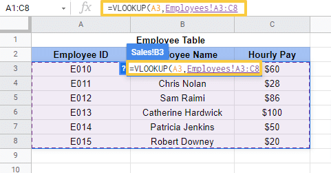
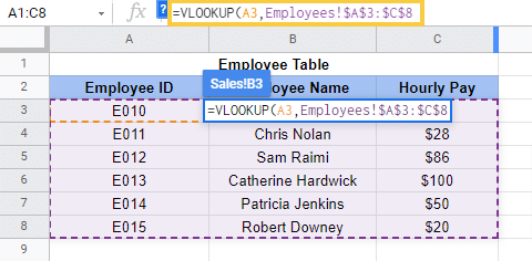
Lock the cell range by pressing F4 (or Ctrl+F4) on your keyboard. This ensures these references won’t change when the formula is copied to other rows within the column. 

The VLOOKUP formula should now show as:

=VLOOKUP(A3,Employees!$A$3:$C$8

Step 4: Input the VLOOKUP index

Add a comma after 8, followed by the column’s index containing the values you want to retrieve. 

Input the number ‘3’ since we’re retrieving the Hourly Rates (the third column in the A3:C8 range). Add the closing parenthesis. 

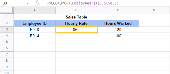
Press Enter, and you should see the Hourly Rate that corresponds to Employee ID E010 in cell B3 in the Sales Sheet. 

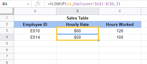
Step 5: Drag down the formula to fill the rest of the cells in the column. 

5. VLOOKUP on Another Sheet in a Separate Spreadsheet File

Doing a VLOOKUP in another Sheet on a separate spreadsheet file uses the same function as the example above.

However, there’s a slightly different second parameter — it includes the IMPORTRANGE function. 

The IMPORTRANGE function is generally used to import values from cells in a separate spreadsheet into your current sheet. 

It includes two parameters:

• spreadsheet_key is the spreadsheet URL you want to import from, and it should be specified in double-quotes (“ “). 
• range_string is a reference to the cell ranges you want to import. It should contain the Sheet name, including the cells you want. For example, if you’re importing cells A3:C8 from the Employees worksheet in the previous example, your range_string should be “Employees!A3:C8”.

Let’s assume you have:

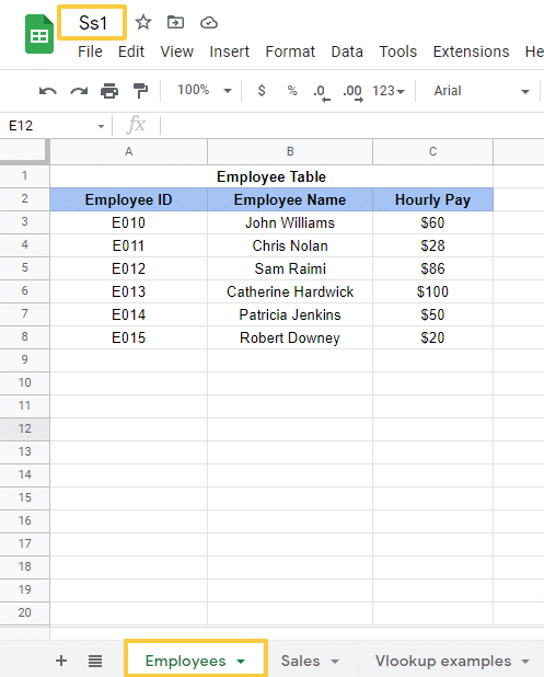
• An ‘Employee’ table in a Sheet named ‘Employees’ within a spreadsheet file called ‘Ss1’
• A ‘Sales’ table in a Sheet named ‘Sales’ within a separate spreadsheet file called ‘Ss2’  

In this example, we’ll retrieve the Hourly Rates that correspond to employee IDs E010 and E014 from the Employees Sheet in Ss1 and display them in cells B3 and B4 on the Sales Sheet in Ss2. 

Here’s how to do it. 

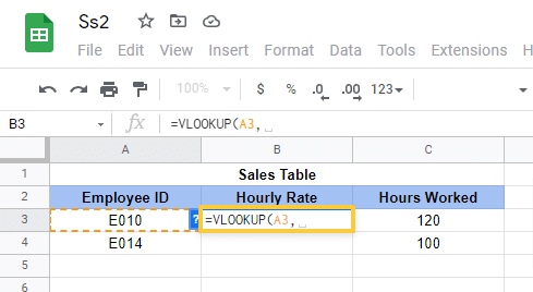
Step 1: Click B3 on the Sales table within Ss2. 

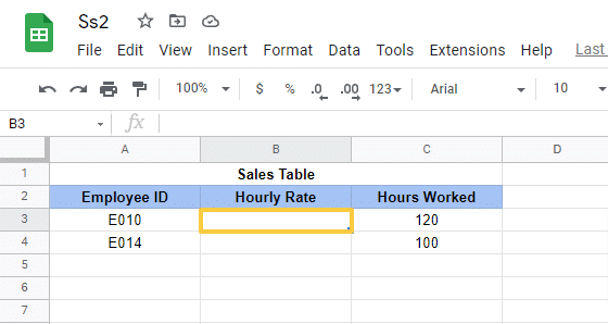
Input =VLOOKUP(, and select cell A3 followed by a comma.

Step 2: Deploy IMPORTRANGE in the formula

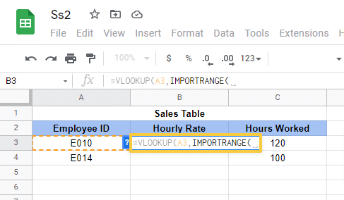
Enter IMPORTRANGE function as the second parameter, then an opening parenthesis. 

Step 3: Open Ss1 and select the Employees Sheet

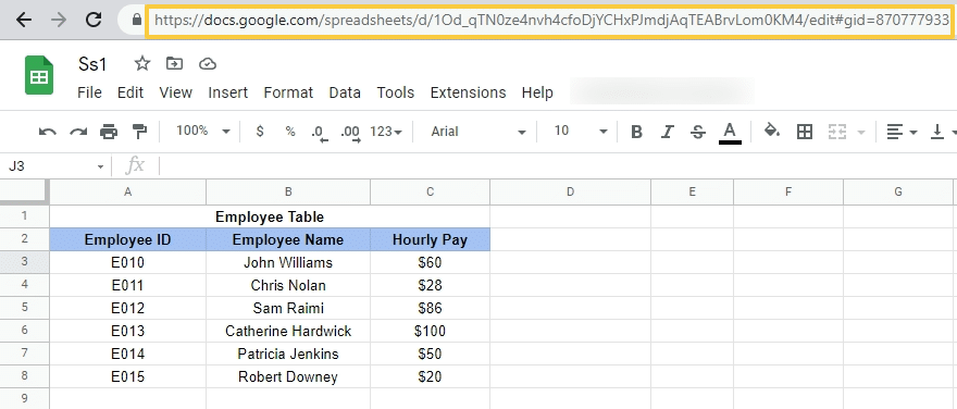
Copy the Google Worksheet’s URL from your browser’s address bar.   

Step 4: Insert URL into IMPORTRANGE

Go back to the Ss2 spreadsheet and paste the URL into the IMPORTRANGE function. Be sure to enclose the URL in double quotes.  

Add a comma after the double quotation mark followed by the source Sheet’s name — ‘Employees’ in this case.  

Step 5: Input Lookup Ranges

Add an exclamation mark (!) and input the cell ranges ($A$3:$C$8) you want to look up from the source Sheet. 

Enclose the entire parameter (source sheet name, exclamation mark, and cell range) in double quotes followed by a comma and closing parenthesis (to close the IMPORTRANGE function). 

The formula is now: 

=VLOOKUP(A3,IMPORTRANGE(“https://docs.google.com/spreadsheets/d/1Od_qTN0ze4nvh4cfoDjYCHxPJmdjAqTEABrvLom0KM4/edit#gid=870777933″,”Employees!$A$3:$C$8”)

Step 6: Add the column index

Add a comma and the column index containing the values you’re retrieving — the Hourly Rates in the third column of the A3:C8 range.

Input the number ‘3’ followed by a closing parenthesis, then press Enter. Now the formula is:

=VLOOKUP(A3,IMPORTRANGE(“https://docs.google.com/spreadsheets/d/1Od_qTN0ze4nvh4cfoDjYCHxPJmdjAqTEABrvLom0KM4/edit#gid=870777933″,”Employees!$A$3:$C$8”),3)

Step 7: Solving #REF! Errors

If you see a #REF! Error, click the Allow access button to connect the Sheets. 

You should now see the hourly rates that correspond to Employee ID E010 in cell B3 of your Sales table. 

Drag down down the formula to fill in the rest of the cells under the column. 

VLOOKUP can be a powerful function once you figure out how to use it to reference information across your Google spreadsheets. Data changes in the original Sheet get automatically updated in your connected cells, making it easy to reference data on multiple Google spreadsheets quickly. 

6. Index match formula for leftward VLOOKUP

The VLOOKUP function cannot search to the left. This means if the search column isn’t the first column in the lookup table, your Google Sheets VLOOKUP won’t work. 

However, you can work around this using a more durable and powerful Index Match formula:

INDEX (return_range, MATCH(search_key, lookup_range, 0))

For instance, you can use this formula: 

=INDEX($F$3:$F$8, MATCH (A3, $G$3:$G$8, 0))

The formula lets you look up the A3 cell value (search_key) in G3:G8 (lookup_range) and return a match from F3:F8 (return_range). 

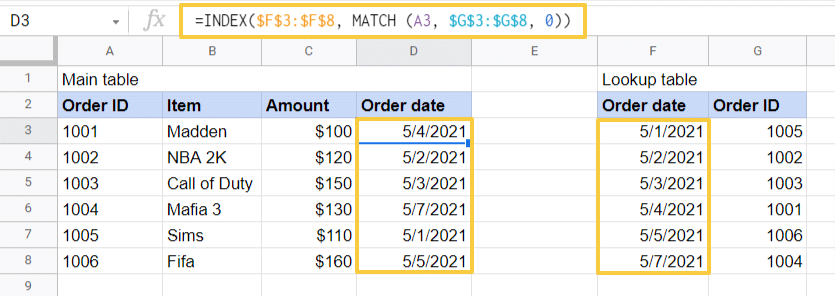
Unlike VLOOKUP, the Index Match formula is unaffected by structural changes within Sheets since it directly references the return column.  

For instance, deleting or inserting a column in your lookup table breaks your VLOOKUP formula since the hard-coded index number becomes invalid. This isn’t the case with Index Match formulas.  

Note: You can generate all of the formulas in this blog automatically using Excelformulabot.

VLOOKUP Eliminates Squint-and-Point Searches for Data

VLOOKUP eliminates the hassle of manually finding and referencing cells in Google Sheets. That’s why Google Sheets users of all backgrounds, from scientists to payroll administrators, consider VLOOKUP indispensable. Although VLOOKUP comes in many iterations, the result is always the same: you save time and energy by avoiding gruntwork. Now you can focus instead on the tasks that really matter.