The Ultimate Guide to Using INDEX in Google Sheets

The Google Sheets INDEX function enables you to lookup and extract data more efficiently in your spreadsheet. 

The INDEX function in Google Sheets returns a cell’s content, specified by row and column offsets. INDEX allows you to easily locate data in your Sheet, and utilize it in other functions.

This is a start-to-finish guide on the Google Sheets INDEX function, from how it works, to use cases, to hands-on examples.  

What does the INDEX function in Google Sheets do?

The Google Sheets INDEX function extracts data from specific cells or cell ranges, based on the row, column, or range you input. The INDEX function then returns the data to the intersection of the specified range. 

Think of the INDEX function like a built-in book index, a quick way to find information (data) on a page (cell) in a book (spreadsheet). 

Syntax of the Google Sheets INDEX function

Let’s look at the INDEX function’s basic syntax to better understand how it works. 

INDEX(reference, [row], [column])

Below is a quick breakdown of each parameter in the INDEX function.

• reference refers to the range of cells you want to extract the data from (or where the data is returned)
• row is the row number within the reference range that you want to extract the data from
• column  is the column number within the reference range that you want to extract the data from

How to use the INDEX function in Google Sheets 

Video Tutorial: How to Use INDEX in Google Sheets (Step-by-Step Guide)

Below are some step-by-step mini-tutorials on how to use the INDEX function in Google Sheets. Also, watch our video tutorial above for a full step-by-step walkthrough on how to use the function.

Let’s use a sample sales information dataset.

Using the Google Sheets INDEX function to return a cell value

You can use the INDEX function to extract data from the specified row and column within the selected range. 

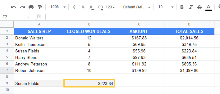
We’ll extract the total sales Susan Fields made from the dataset in this example. Select the A2:D7 as the range of cells. 

Susan Fields’ data is in the third row, and the total sales amount is in the fourth column.

To find out Susan Fields’ total sales, your INDEX formula should be:

=INDEX(A2:D7,3,4)

The result will show Susan Fields’ total sales. 

Harness the same formula to return other cell values in the table by changing the parameters of the INDEX function. 

Let’s try another example. This time, we’ll retrieve Robert Johnson’s closed won deals using this formula: 

=INDEX(A2:D7,6,2)

The INDEX function should show the following results: 

And that’s how you use the INDEX function to return a cell value in Google Sheets. 

AI + Google Sheets: Use Formula Builder to Automatically Generate INDEX Formulas

You can also use Coefficient’s free Formula Builder to automatically create the formulas in this first example. To use Formula Builder, you need to install Coefficient. The install process takes less than a minute.

We’ll outline how to install Coefficient from the Google Workspace Marketplace. Or you can skip the marketplace altogether, and get started for free right from our website. 

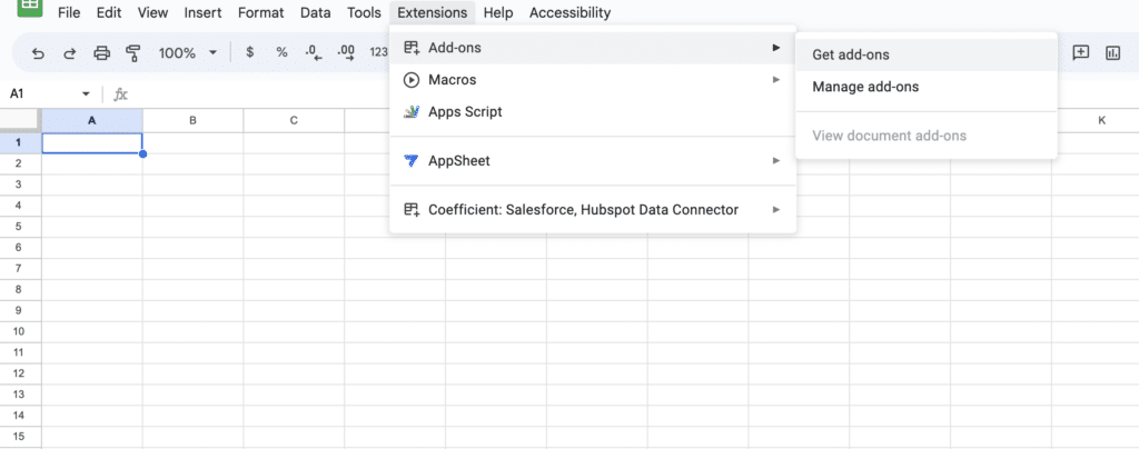
First, click Extensions from the Google Sheets menu. Choose Add-ons -> Get add-ons. This will display the Google Workspace Marketplace. Here a direct link to Coefficient’s Google Workspace Marketplace listing. 

Search for “Coefficient”. Click on the Coefficient app in the search results.

Accept the prompts to install. Once the installation is finished, return to Extensions on the Google Sheets menu. Coefficient will be available as an add-on.

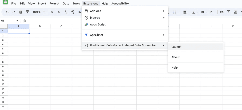
Now launch the app. Coefficient will run on the sidebar of your Google Sheet. Select GPT Copilot on the Coefficient sidebar.

Then click Formula Builder.

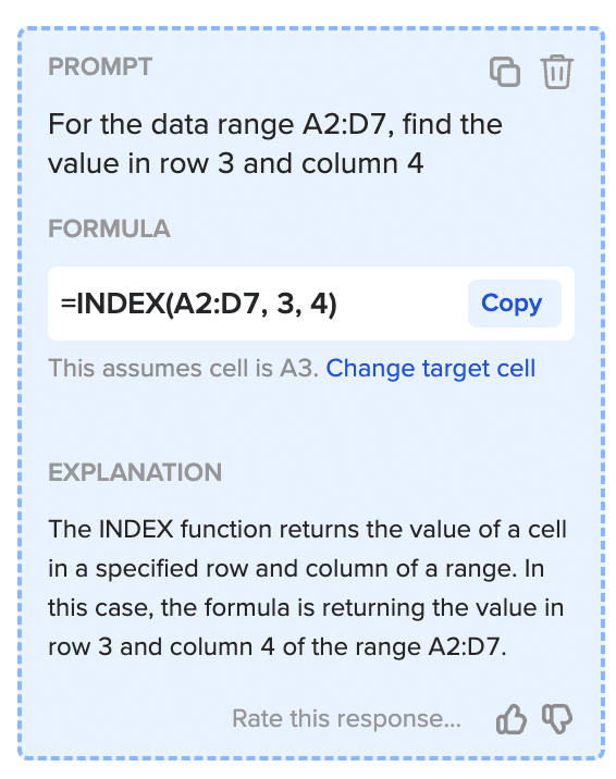
Type a description of a formula into the text box. For this example, type: For the data range A2:D7, find the value in row 3 and column 4.

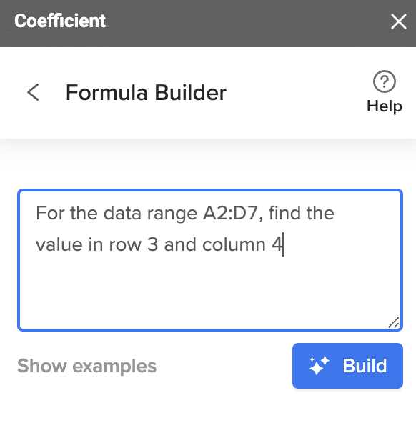
Then press ‘Build’. Formula Builder will automatically generate the formula from the first example.

Using the INDEX function to return an array formula

Besides retrieving one cell’s value, the INDEX function also enables you to extract an entire row of cells.  

Let’s retrieve all of Harry Stone’s complete row of sales information. We’ll extract all four cells on the fourth row of the table.  

Use the INDEX function to return an array formula containing the fourth row’s four values. The formula is the following:

=ArrayFormula( INDEX (A2:D7,4,0) )

4 refers to the row number, and 0 is the column number where the data we want to retrieve resides. 

Select the cell where the results should appear. It should be adjacent to cells that can contain all your extracted values. For this example, you will need 3 empty cells to the right of the cell with the INDEX formula.

Input the formula in your selected cell and press Enter. 

Your returned data should look like this:

Using the INDEX Function to extract data columns

You can extract all the cell values of a column within your cell range using the Google Sheets INDEX function. 

Suppose you want to extract the names of all your sales reps in this dataset. The formula to do this is:

= ArrayFormula (INDEX(A2:D7,0,1))

Select a cell within the column where the results should appear (cell A9 in this example). Input the formula and press Enter. 

The results should show a new column containing the names of your sales reps. 

How to use the INDEX function in other Google Sheets formulas

You can leverage INDEX alongside other formulas and functions, as seen in the examples below.  

Using INDEX with the COUNTA function

Together, the COUNTA and INDEX functions can calculate values using the last row of data within a list or table that is updated regularly. 

Let’s use a simple table showing sales data with weekly updates. 

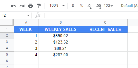
Use the formula below to perform regular calculations using the most recent week’s average sales. 

=INDEX((A:B), COUNTA(A:A),2)

The results should look like this. 

Let’s break down the syntax of the combined formulas. 

• Columns A and B are the range 
• The COUNTA(A:A)function counts the number of data points within column A 
• The INDEX formula takes the number or value that COUNTA(A:A)counted as the row it extracts the results from  
• 2 tells the formula to get the result from the data range’s column (column B in this example)

This combined INDEX and COUNTA formula returns the most recent row of your weekly sales data.  

Combining the MATCH and INDEX functions 

Using the INDEX and MATCH functions together is one of the most powerful ways to look up values in your Google sheet. 

While you can use VLOOKUP, the function has limitations. We’ll go over these limitations to see why using a MATCH INDEX function is easier and more efficient, including when best to use the combination. 

First, let’s apply VLOOKUP to this sample sales rep data to show how the function works. 

How to use the VLOOKUP function

Retrieve the name of the sales rep with Employee ID 161 using this VLOOKUP formula:

=VLOOKUP(161,A2:B11,2,FALSE)

This is the result.

The VLOOKUP formula (in cell D2) looks up 161 in the Employee ID column since it’s the leftmost data within the A2:B11 range. Then the function retrieves the value within the second column (column B) of the row, assuming the data isn’t sorted.

However, the VLOOKUP function can only look up values in the leftmost column of the table and reference static cells. Let’s try inserting a new column containing the sales reps’ locations between the first and second columns  (A and B). 

The returned lookup value now shows “DE” instead of “Sarah”, since VLOOKUP is a semi-static formula. Google Sheets updated the second parameter to reflect the range we added, but it did not change the column index (the third parameter) accordingly.  

VLOOKUP also cannot look up values from columns that are not in the leftmost part of the cell range. For instance, suppose an Employee ID column is on the rightmost part of the table.

You could move the Employee ID column to the leftmost part of your table. However, doing this isn’t always ideal, especially with presentation specifications and data layouts that don’t let you rearrange the columns. 

This is where INDEX and MATCH formulas come in handy. 

Using the INDEX and MATCH functions 

Before blending the INDEX and MATCH function, let’s go over how a MATCH function in Google Sheets works first.

Essentially, the MATCH function scans your dataset for a specific value and returns its position with this syntax. 

=MATCH(search_key, range, [search_type])

• search_key is the record or value you want to find 
• range refers to the column or row you want the function to search
• search_type is an optional parameter that defines whether the match should be approximate or exact. If omitted, the default is one (1). 

1 means sorting the range in ascending order, and the function retrieves the largest values that are less than or equal to the search_key. 

0 tells the function to look for the exact match in unsorted data ranges. 

-1 indicates that values are ranked by descending sorting order, which tells the function to get the smallest value greater than or equal to the search_key. 

For example, to get George’s position in this sales rep dataset, use this MATCH function formula:

=MATCH(“George”, A1:A10, 0)

Here’s the result:

Unlike the INDEX function, the MATCH function is performed within a single column or row. The MATCH function finds the location of the defined value. 

Now that we know how to use the MATCH function let’s move on to the INDEX MATCH function. 

Syntax: 

INDEX(reference, MATCH(search_key, range, search_type))

Both cell ranges selected for the INDEX and MATCH functions must be in a single column. 

The combination is similar to executing a VLOOKUP, except you specify the columns to search, and return the value in separate ranges. However, you won’t encounter the errors that VLOOKUP generates.

Use the MATCH function to see which row contains Employee ID 161 within column C. This will return a number that tells the INDEX function what row within column A to search for the sales rep. 

The formula should look like this:

=INDEX(A2:A11,MATCH(161,D2:D11,0))

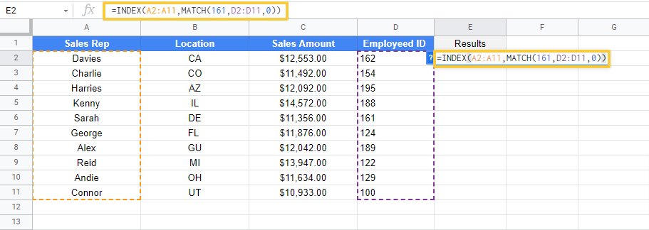
The result shows you the name of Employee ID 161 (Sarah). 

Unlike VLOOKUP, the INDEX MATCH combination function works even if the lookup column (Employee ID) isn’t the leftmost column. It also works like VLOOKUP when the lookup column is the leftmost in the table. 

Now let’s add another column to test the versatility of the INDEX MATCH function. Add a new column between the Location and Sales Amount columns. And voila: Google Sheets automatically updates the cell references to accommodate the change.

Using the MATCH and INDEX functions together is more flexible than VLOOKUP.  

You can make the INDEX MATCH combination function even more powerful by using two MATCH functions instead of one. 

Let’s use the sample bi-dimensional array of data you want to retrieve value from. But this time, use the MATCH function twice within the INDEX function. The sample data shows the monthly average temperature from 2015 to 2020.  

Pull the average temperature for a specific month and particular year from the array using this formula: 

=INDEX(B2:M7, Match(B11, A2:A7, false), Match(B10, B1:M1, false))

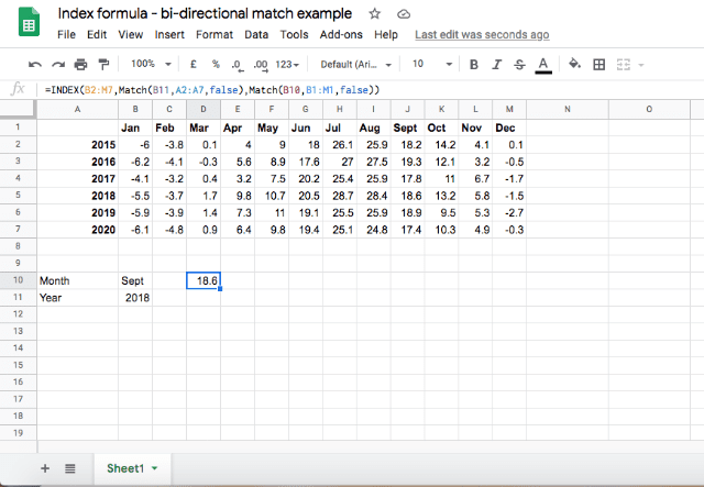
The combination function retrieves the row’s location for the proper year (2018, the fourth data row). This also retrieves the column for the right month (September, the 9th data column). The INDEX function takes the coordinates and returns the average temperature for September 2018 (18.6). 

Now you understand why the combo of INDEX and MATCH often outperforms VLOOKUP. 

Google Sheet INDEX Function: The Book Index for Your Spreadsheet

The INDEX function in Google Sheets is a quick and efficient built-in method for retrieving data in your spreadsheet. Once you master the basics, you can combine INDEX with other Google Sheets capabilities to build out more powerful data lookup functions that extract data in a faster way.    

For more spreadsheet tips, check out our other Google Sheets tutorials: 

• How to Use the Google Sheets QUERY Function
• The Ultimate Guide to Using Pivot Tables in Google Sheets
• Linking Data Between Multiple Google Sheets: Ultimate Guide
• The Ultimate Guide to VLOOKUP in Google Sheets