Ultimate Guide to XLOOKUP in Google Sheets (Updated August 2022)

XLOOKUP is a function in Google Sheets and Microsoft Excel that can identify values in an array or range quickly. The function is more versatile than LOOKUP, VLOOKUP, and HLOOKUP.  XLOOKUP first came to Excel in 2019 and Google Sheets in August 2022.

XLOOKUP supports exact and approximate matching, lookups in vertical and horizontal ranges, and wildcards for partial matching. Read on, or watch our video walkthrough, to learn how to use this modern lookup function to effectively replace VLOOKUP, HLOOKUP and INDEX-MATCH in your formulas.

Video Walkthrough: How to Use XLOOKUP (Step-by-Step Guide)

What is the XLOOKUP function?

The XLOOKUP function allows you to search any row or column for a specific search term or value and then return a related cell’s value from a parallel row or column. The function is an improvement on VLOOKUP and HLOOKUP, offering easier usage as well as advanced settings.

Now that you know how the XLOOKUP function works in Excel, let’s look at several examples of alternative options in Google Sheets.

XLOOKUP function syntax

The XLOOKUP function syntax in Google Sheets looks like this:

=XLOOKUP(search_key, lookup_range, result_range, [missing_value], [match_mode], [search_mode])

The function includes three required and three optional arguments.

Required arguments:

• search_key is the value you want to find
• lookup_range refers to the array containing your lookup_value
• result_range is the array that contains the corresponding return value

Optional arguments:

• [missing_value]is returned when the lookup_value isn’t found. The formula returns an #N/A error if you don’t specify this argument.
• [match_mode]enables you to specify your preferred type of match, such as:
  • 0, which is the default option (exact match). Use this if you want the lookup_value to match the value in your lookup_array. 
  • -1 finds the exact match but returns the next smallest value or item.
  • 1 identifies the exact match but returns the next largest value or item. 
  • 2 allows your formula to conduct partial matching using wildcard characters, such as a star (*) or a tilde (~). 
• [search_mode] defines how the XLOOKUP function should find the value (or item) in the lookup_array. 
  • 1 is the default option that tells the function to search for the lookup_value from top to bottom in the lookup_array.
  • -1 tells the function to search from the bottom to the top. It’s useful when searching for the last matching value in the lookup_array.
  • 2 allows the function to conduct a binary search when you want the data in ascending order. Not sorting can result in the wrong result and errors. 
  • -2 lets the function perform a binary search if you want the data sorted in descending order.

The benefits of using the XLOOKUP function

Below are several advantages of using the XLOOKUP function.

• XLOOKUP can find exact matches by default. Other functions, such as VLOOKUP, require including FALSE as the last parameter to get the right result. 
• XLOOKUP makes it easy to specify a value for when there is no match returned. Simply add the value as the 4th argument, if desired, like so: =XLOOKUP(G6,A:A,C:C,”No Match Found”)
• XLOOKUP includes optional parameters. If you want to search for special situations, such as searching for a value when you only know some parts of it, you can use XLOOKUP for wildcard searches, including an asterisk star “*” to represent any zero or more characters. Use a question mark “?” to represent any single character. For example, you can lookup “F*” to return any matches where the text string begins with “F”.
• XLOOKUP returns references as output. XLOOKUP can return references, which means you can combine XLOOKUP output with other formulas in many innovative ways. 
• XLOOKUP can search in any direction. HLOOKUP can only search in the topmost row, and VLOOKUP can only search values in your table’s leftmost column. XLOOKUP doesn’t have this limitation. The function gives you more flexibility since it can search right or left and top or bottom.  
• XLOOKUP lets you return multiple values. You can manipulate the result_range perimeter in your XLOOKUP formula to pull an entire column or row of data related to your lookup value.  
• XLOOKUP allows you to search with multiple criteria. XLOOKUP can handle arrays natively, making it possible to search values or cells with multiple criteria. 
• XLOOKUP allows you to insert, change, or delete columns. Other LOOKUP functions, such as VLOOKUP, have formulas that can break when you add or remove columns. 

For an overview of how XLOOKUP differs from VLOOKUP, watch our video tutorial below.

Video Tutorial: XLOOKUP vs. VLOOKUP

XLOOKUP Examples in Google Sheets

Here are some examples of how to leverage XLOOKUP, based on popular use cases. Also, watch our video walkthrough below for a full step-by-step guide to using XLOOKUP.

In this first example, let’s say you want to look up the name “Jacob” from cell G4 (search key) in the range A:A (lookup range) and return the value found in range D:D (result range) from the same row as Jacob (row 4 in this case).

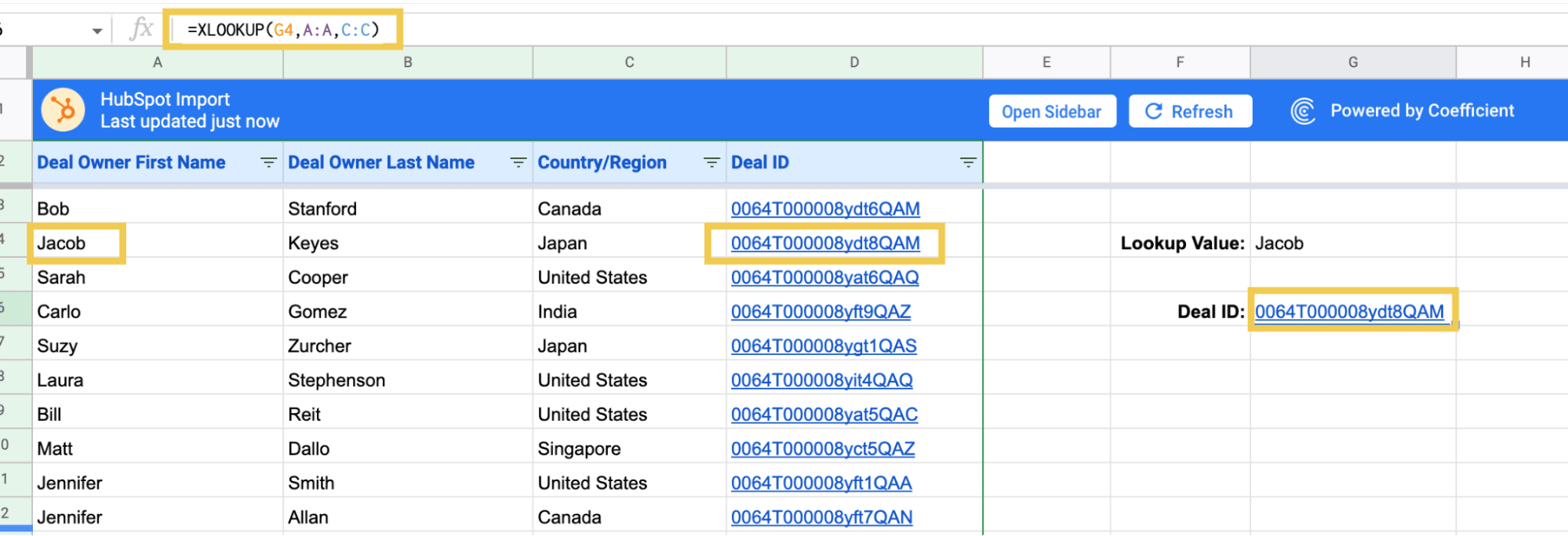
Note: Using VLOOKUP, this formula would’ve been =VLOOKUP(G4,A:D,4,FALSE)

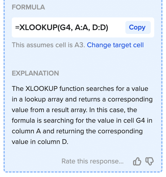
AI + Google Sheets: Use Formula Builder to Automatically Generate XLOOKUP Formulas

You can also use Coefficient’s free Formula Builder to automatically create the formulas in this first example. To use Formula Builder, you need to install Coefficient. The install process takes less than a minute.

We’ll outline how to install Coefficient from the Google Workspace Marketplace. Or you can skip the marketplace altogether, and get started for free right from our website. 

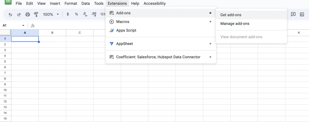
First, click Extensions from the Google Sheets menu. Choose Add-ons -> Get add-ons. This will display the Google Workspace Marketplace. Here a direct link to Coefficient’s Google Workspace Marketplace listing. 

Search for “Coefficient”. Click on the Coefficient app in the search results.

Accept the prompts to install. Once the installation is finished, return to Extensions on the Google Sheets menu. Coefficient will be available as an add-on.

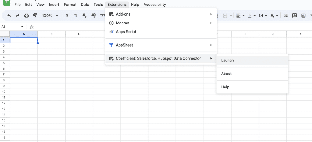
Now launch the app. Coefficient will run on the sidebar of your Google Sheet. Select GPT Copilot on the Coefficient sidebar.

Then click Formula Builder.

Type a description of a formula into the text box. For this example, type: Find cell G4 in lookup range A:A and result range D:D.

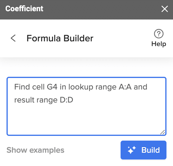
Then press ‘Build’. Formula Builder will automatically generate the formula from the first example.

Simple exact value lookup by row

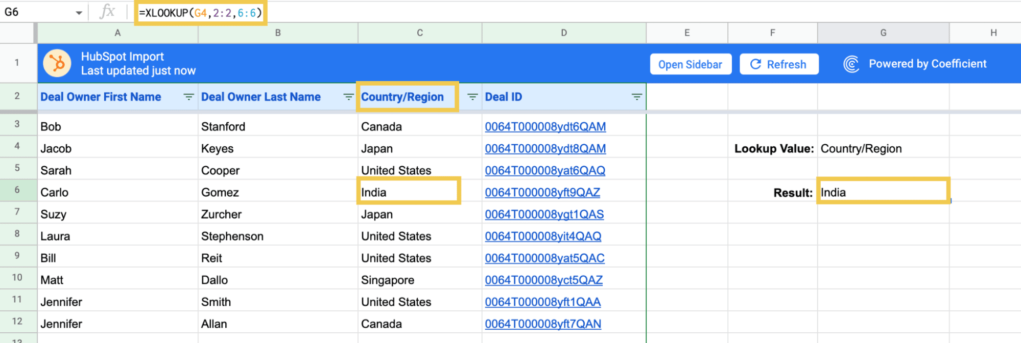
As mentioned, XLOOKUP also replaces HLOOKUP, which searches horizontal rows, instead of vertical columns, as VLOOKUP does. 

In this next example, let’s replace Jacob’s name with the column header name from C2, “Country/Region”. 

Now let’s search row 6 and find the associated Country name from Column C. 

We can easily change our search term (G6) to be “Deal Owner Last Name”, and the formula will return “Gomez” from the same row instead.

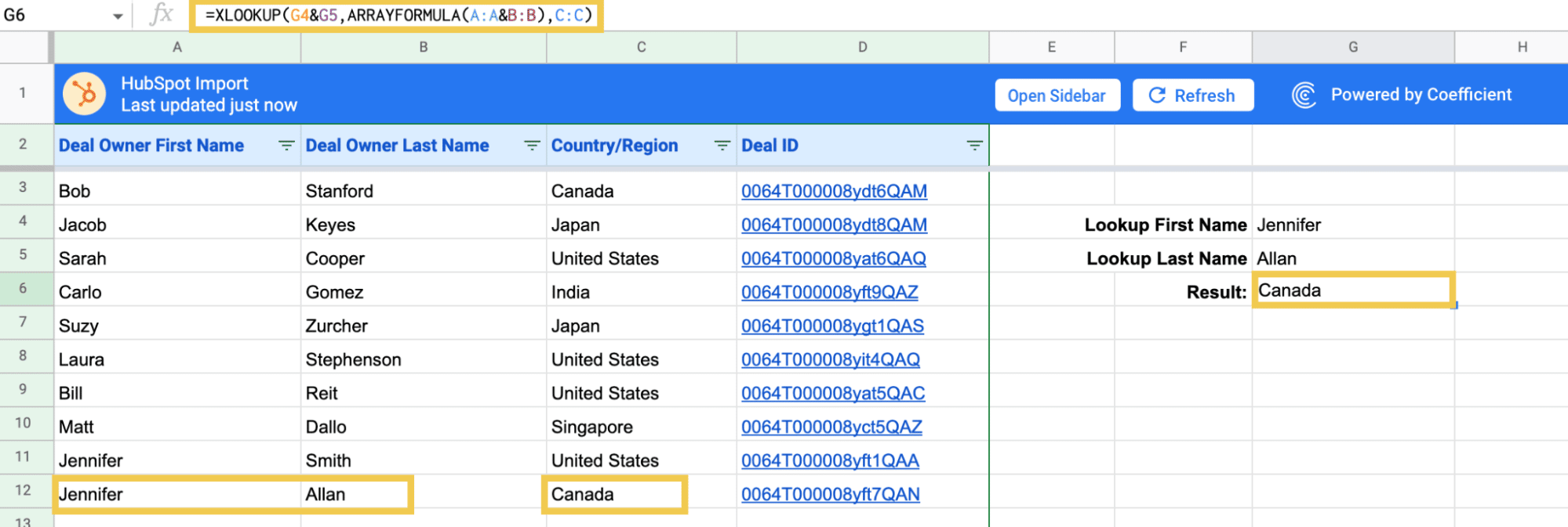
Search Multiple Terms or Conditions with XLOOKUP

Like other Lookup formulas, if there are multiple matching values found in the lookup range, XLOOKUP will return the result for the first match (unless you are using non-exact match searches). 

In the example above, if we searched for “Jennifer”, we would only be able to see the related values for the first match, “Jennifer Smith”.

To be able to narrow down our results to the correct match, it can be helpful to combine multiple criteria. The best way to do this in XLOOKUP formulas is use a simple Array Formula like this:

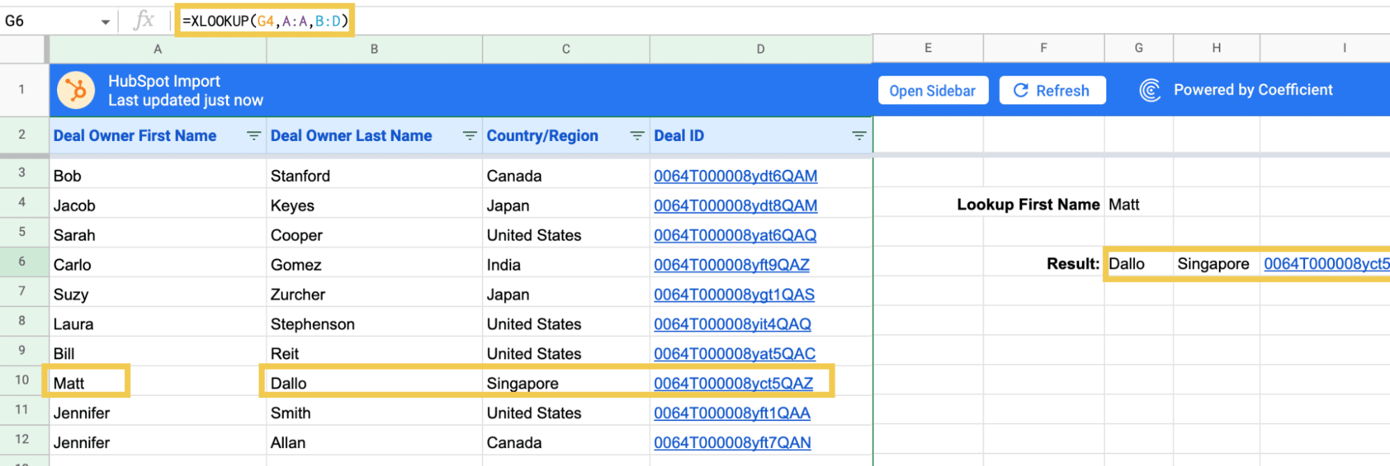
Returning Values From Multiple Columns or Rows with XLOOKUP

Now let’s say you would like to search for a First Name and return all of the values from the same row. 

The obvious way to do this might be to have multiple VLOOKUP or XLOOKUP formulas, each returning one value.

But XLOOKUP actually makes this much easier. You can do this all in one formula by specifying a Result Range that is multiple columns:

XLOOKUP alternatives in Google Sheets

XLOOKUP with INDEX MATCH

You can combine the Google Sheets INDEX and MATCH functions to simulate the functionality of XLOOKUP.

The INDEX function returns the content of the cell or cells around it. The function has the following syntax:

=INDEX(reference, [row], [column])

The MATCH function returns the position of the cell matching the given value or key within a range. The function’s syntax is:

=MATCH(search_key, range, [search_type])

Since the MATCH function returns the given value’s relative position (or index), you can substitute it for the row index within the INDEX function.

The INDEX MATCH formula syntax becomes:

=INDEX(reference, MATCH(search_key, range, search_type), [column])

To apply this to the sample dataset, index the range containing the value you want to return (the Deal ID).

Free AI-Powered Tools Right Within Your Spreadsheet

Supercharge your spreadsheets with GPT-powered AI tools for building formulas, charts, pivots, SQL and more. Simple prompts for automatic generation.

Then use the MATCH function in Google Sheets to return the correct row using the lookup value within cell F3.

Include the FALSE (or 0) arguments at the end to exactly match the name within cell F3 to the name in your lookup table.

Your whole INDEX MATCH formula should look like this:

=INDEX(C3:C11,MATCH(F3,A3:A11,0))

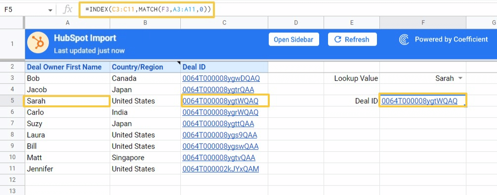
The INDEX MATCH combination in Google Sheets works in the same way as XLOOKUP in Excel.

XLOOKUP with FILTER function

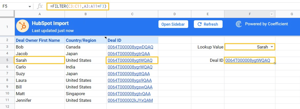
The FILTER function is one of the easiest ways to replicate XLOOKUP in Google Sheets. Here’s the basic FILTER function syntax.

=Filter(return_array, lookup_array=lookup_value)  

Specify the range containing the value you want to search or return (C3:C11). Then add the criteria range (A3:A11) and criteria (F3) to your formula.

The FILTER formula to replace XLOOKUP is:

=FILTER(C3:C11,A3:A11=F3)

You can also use the filter function to do more sophisticated lookups, such as:

• Defining conditions based on more than one variable
• Set more advanced conditions, such as when text starts or ends with different characters
• Return and sort a list

XLOOKUP with VLOOKUP

XLOOKUP is essentially a more robust and flexible version of VLOOKUP. However, you can leverage VLOOKUP in Google Sheets to replicate the functionality of XLOOKUP.

VLOOKUP’s syntax in Google Sheets is as follows:

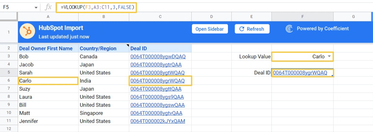
=VLOOKUP(search_key, range, index, [is_sorted])

Begin by specifying the search_key in our dataset (F3). Next, select all the data (A3:C11) and specify the column number you want to return.

In our example, we want to retrieve the Deal ID of a specific Deal Owner, located in column three. We’ll end our formula with a FALSE argument to ensure an exact match with Deal Owner First Name.

The VLOOKUP formula will look like this:

=VLOOKUP(F3,A3:C11,3,FALSE)

XLOOKUP with QUERY function

The QUERY function allows you to write SQL-type queries in Google Sheets. You can deploy a query to perform a lookup function.

Quick note: QUERY formulas are more complex than the other XLOOKUP alternatives we’ve outlined.

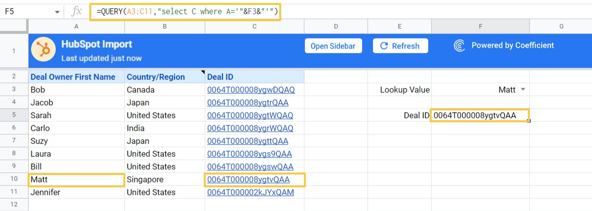
Let’s perform a lookup in Google Sheets by utilizing the following query:

=QUERY(the_whole_table, “select C where A='”&lookup_value&”‘”)

First, specify the entire data range (A3:C11).

Then add a SELECT statement to specify the column you want to return (Column C).

Finally, provide the criteria for your query: return column C when column A is equal to cell F3’s value.

Your QUERY formula should look like this:

=QUERY(A3:C11,”select C where A='”&F3&”‘”)

One downside to using the QUERY function is its hard-coded column labels, like VLOOKUP. If you change the table, the formulas can break.

Harness the power of XLOOKUP in Google Sheets

Move over, Excel! XLOOKUP is a long awaited function for Google Sheets power users. Now it’s finally here. Give it a try now! And stay tuned as we release more walkthroughs on the new Google Sheets functions.