SUMIFS Google Sheets: Ultimate Guide

The SUMIFS function in Google Sheets enables you to sum values in your spreadsheet based on predefined conditions.

Unlike the SUMIF function, which adds values to a sum based on a single condition, SUMIFS can enforce two or more conditions. The Google Sheets SUMIFS function only adds a value to a sum when all these conditions are met.

This ultimate guide to SUMIFS in Google Sheets will show you how to master the function through a series of sample formulas, example use cases, and step-by-step walkthroughs. Also, watch our video tutorial below for a full overview of the Google Sheets SUMIFS function.

Video Tutorial: How to Use SUMIFS in Google Sheets

Why use the SUMIFS function in Google Sheets?

In Google Sheets, the most basic way to get the sum of cell values is to create an additive formula. 

=B1+B2+B3+B4+B5

However, this rudimentary method isn’t practical when adding longer ranges of cells, such as entire rows or columns. That’s what SUM is for. But SUM isn’t feasible when you only want to sum certain values within a range. 

SUMIFS is a better option in such cases. Think of SUMIFS as a SUM function with superpowers. With SUMIFS, you can calculate sums across ranges easily, and define criteria to exclude certain values from the sum.  

Syntax of the Google Sheets SUMIFS function

The basic syntax of the SUMIFS function looks like this:

SUMIFS(sum_range, criteria_range1, criteria1, [criteria_range2, criteria2], …)

The syntax consists of the following arguments:

• Sum_range is the range of cells you want to sum.

• Criteria_range1 is the range of cells you want to test with your criteria. 

• Criteria1 defines the criteria for the cells in Criteria_range1. The cells that meet the criteria are added to the sum.

• Criteria_range2, criteria2, … represent additional ranges and criteria within a SUMIFs function. You can include a maximum of 127 range/criteria pairs per formula. 

Each SUMIFs formula must define at least one range/criteria pair, although in that case, a SUMIF formula can accomplish the same operation.  

Key tips for using SUMIFS function in Google Sheets

While implementing SUMIFS formulas in Google Sheets is relatively straightforward, consider these key tips to ensure a smooth process. 

• SUMIFS only adds cell values that meet all the defined criteria, similar to the logical operator AND in programming languages. 

• You must enclose dates, text, and wildcard characters in quotation marks.

• Criteria_ranges must not exceed the Sum_range, or the SUMIFS formula will result in a #VALUE error.

• You need to insert logical operators in double-quotes within text, numbers, and dates.

These tips will allow you to steer clear of the most common errors we’ve seen users make. Now onto the examples. 

How to use the SUMIFS function in Google Sheets

Before using SUMIFS formulas, let’s set up a sample dataset first. For this example, we’ll import sales data from HubSpot to Google Sheets using Coefficient. The Coefficient app lets you automatically sync data from your business systems with Sheets. 

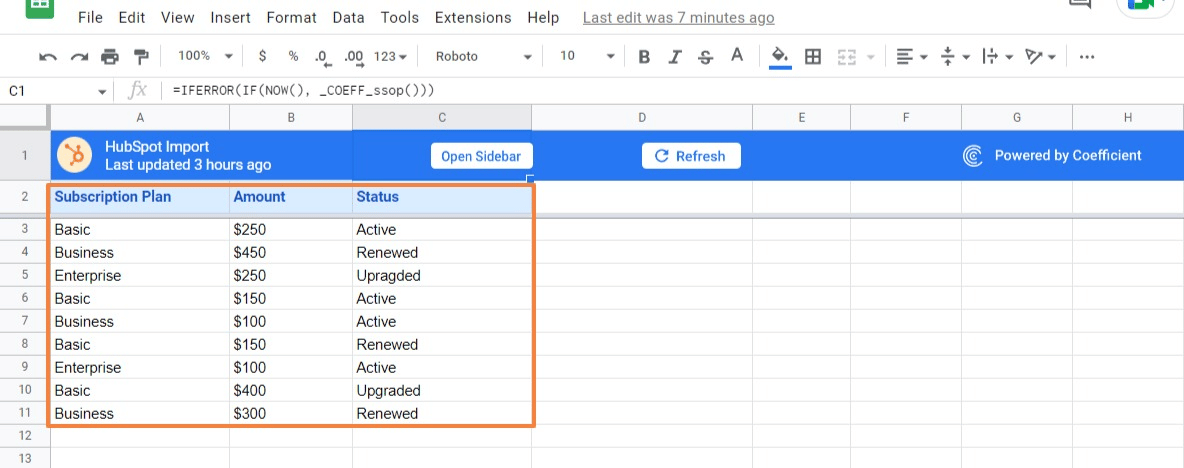
Now let’s use this real-life data set to learn how to use the SUMIFS function. Let’s say you want the total amount for a specific item with a certain subscription status, such as Active Basic plans. 

In theory, you could use an arrayformula that looks like this:

=ARRAYFORMULA(SUMPRODUCT((A6:A14=”Basic”)*(C6:C14=”Active”)*(B6:B14)))

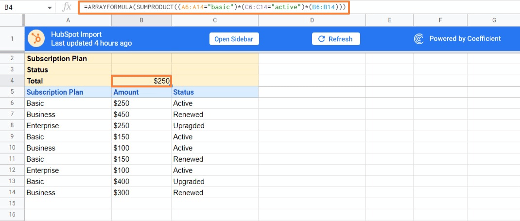
While using an ARRAY formula gives your expected result, it can be needlessly complex. An easier method is to use the Google Sheets SUMIFS function. 

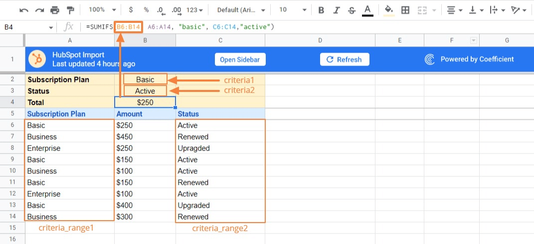
Let’s define the arguments in the SUMIFS formula. We only want to add values associated with Active Basic plans:

• Criteria_range1 is A6:A14, and criteria1 is “Basic”.
• Criteria_range2 is C6:C14, and criteria2 is “Active”. 
• The Sum_range is B6:B14, since the values we want to sum are in column B. 

The entire SUMIFS formula will look like this:

=SUMIFS(B6:B14, A6:A14, “basic”, C6:C14,”active”)

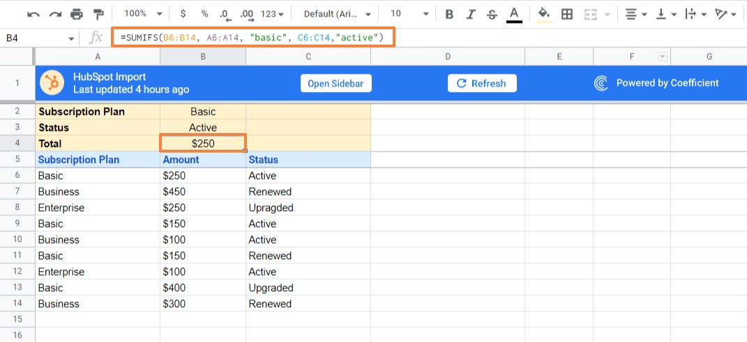
The final result corresponds to each argument in the formula:

Use GPT Formula Builder to Automatically Generate SUMIFS Formulas

You can use Coefficient’s free Formula Builder to automatically create your SUMIF formulas for you. To use Formula Builder, you need to install Coefficient by following along with the prompts. The install process takes less than a minute.

Once the installation is finished, return to Extensions on the Google Sheets menu. Coefficient will be available as an add-on.

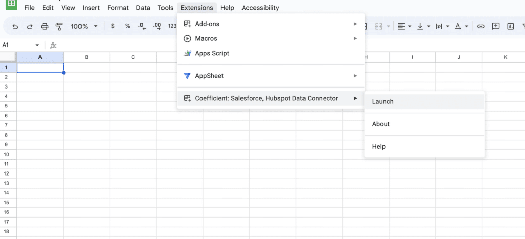
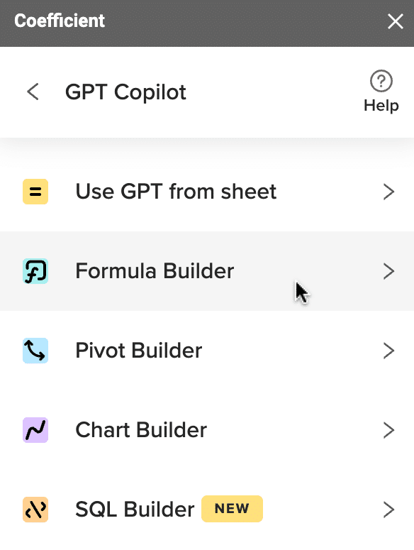
Now launch the app. Coefficient will run on the sidebar of your Google Sheet. Select GPT Copilot on the Coefficient sidebar.

Then click Formula Builder.

Type a description of a formula into the text box. For this example, type: Add the value in B6:B14 if the value in A6:A14 is “basic” and the value in C6:C14 is “active”.

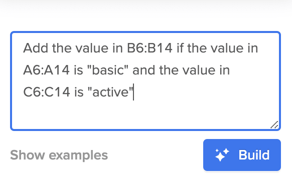
Then press ‘Build’. Formula Builder will automatically generate the formula from the first example.

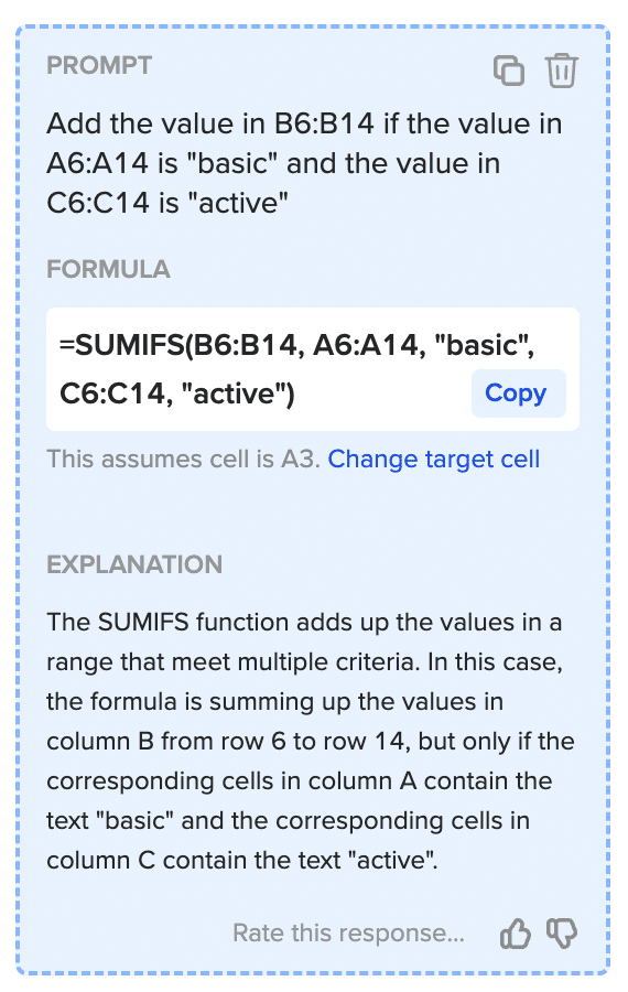
Simply copy-paste your SUMIF formula in the desired cell.

Now that we know the basics, let’s go over several other examples of using SUMIFS formulas with different criteria types.  

Using a SUMIFS function with logical operators

You should use comparison operators when SUMIFS criteria refer to dates or numbers. Here’s a refresher on how to deploy comparison operators in Google Sheets: 

• Greater than (>)
• Less than (<)
• Greater than or equal to (>=)
• Less than or equal to (<=)
• Equal to (= or omitted)
• Not equal to (<>)

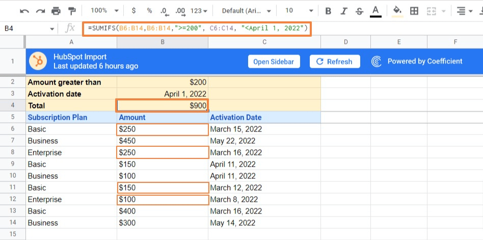
The SUMIFS formula below identifies subscriptions active before April 1st, 2022, and sums the values greater than or equal to 200. 

=SUMIFS(B6:B14,B6:B14,”>=200″, C6:C14, “<April 1, 2022”) 

If you want to replace values with cell references, enclose the logical operator in quotation marks. Also, use an ampersand to concatenate the reference cell. 

Your formula will look like this:

=SUMIFS(B6:B14,B6:B14,”>=”&B1, C6:C14, “<“&B2)

Using SUMIFS with blank and non-blank cells

You can also sum numbers in one column if a cell in a separate column is empty. Here’s how:

• “=” to sum blank cells (empty)
• “” to sum empty cells (including zero-length strings)
• “<>” to add non blank cells (including zero-length strings)

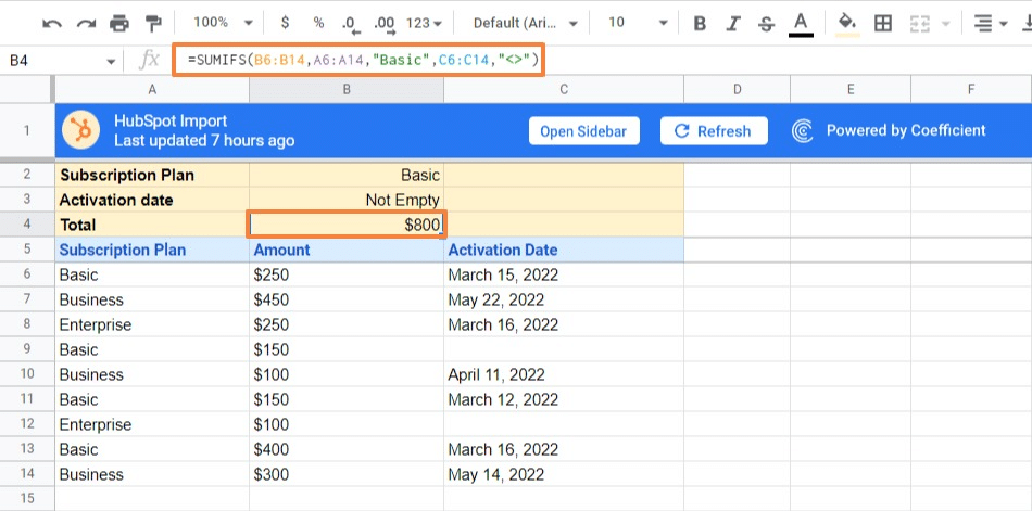
Let’s say the Activation Date column has empty cells. You can write a SUMIFS formula to sum Basic plans with set activation dates, based on the empty cells:

=SUMIFS(B6:B14,A6:A14,”basic” ,C6:C14, “<>”)

Using SUMIFS with other functions

The conditions in a SUMIFs formula can use other functions as dependencies. In other words, you can embed other functions in the SUMIFS formula’s criteria. 

Let’s say we want to include activation dates from today. In this case, we can concatenate the less than or equal to operator (<+) with the TODAY () function inside the SUMIFS formula:

=SUMIFS(B6:B14,A6:A14, B2,C6:C14, “<=”&TODAY()) 

Using SUMIFS with multiple OR criteria in the same column

You can add two SUMIFS functions together as well. For instance, if you want to sum the values for “Basic” or “Enterprise” plans, you can use a SUMIFS() + SUMIFS() combination:

=SUMIFS(B:B,A:A,”basic”) + SUMIFS(A:A,”business”,B:B)

If there are three or more criteria, you should opt for a more compact formula. Include the items in an inline array. Use ArrayFormula to produce each item’s subtotal, and wrap everything in a SUM() function to add the subtotals.

The formula will look like this:

=SUM(ARRAYFORMULA(SUMIFS(A6:A14, {“basic”, “business”, “enterprise”}, B6:B14)))

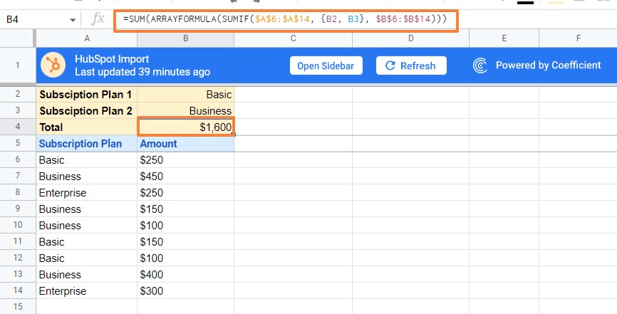
Now enter the items in individual cells. Include cell references for your array (for non-contiguous cells) or supply a range (for contiguous cells). We’ll narrow the list to these two items:

=SUM(ARRAYFORMULA(SUMIFS(A6:A14, {B1, B2}, B6:B14)))

Or

=SUM(ARRAYFORMULA(SUMIFS(A6:A14, B1:B2, B6:B14)))

If you want, you can add up subtotals using the SUMPRODUCT function instead of an ArrayFormula:

=SUMPRODUCT((A6:A14=”basic”) + (A6:A14=”business”), B6:B14)

Use this syntax for multiple OR criteria (with three or more items):

=SUMPRODUCT((A6:A14={“basic”, “business”}) * B6:B14)

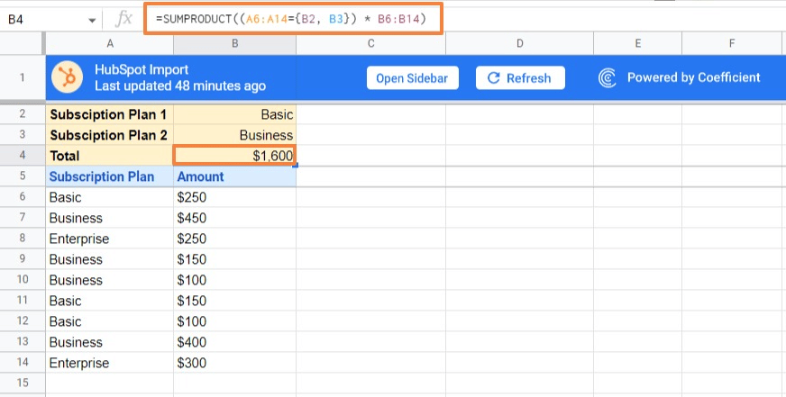
Replace the array elements with cell references, and you’ll get a more compact formula.

=SUMPRODUCT((A6:A14={B1, B2}) * B6:B14)

Using SUMIF with OR criteria and results in other cells

As shown above, you can generate each item’s subtotal in a different cell with an array formula. From there, you can adjust the cell references and remove the SUM() part, so the formula looks like this:

=ARRAYFORMULA(SUMIFS(A4:A13, {“basic”, “business”, “enterprise”}, B4:B13))

In this example, the formula will produce the following results:

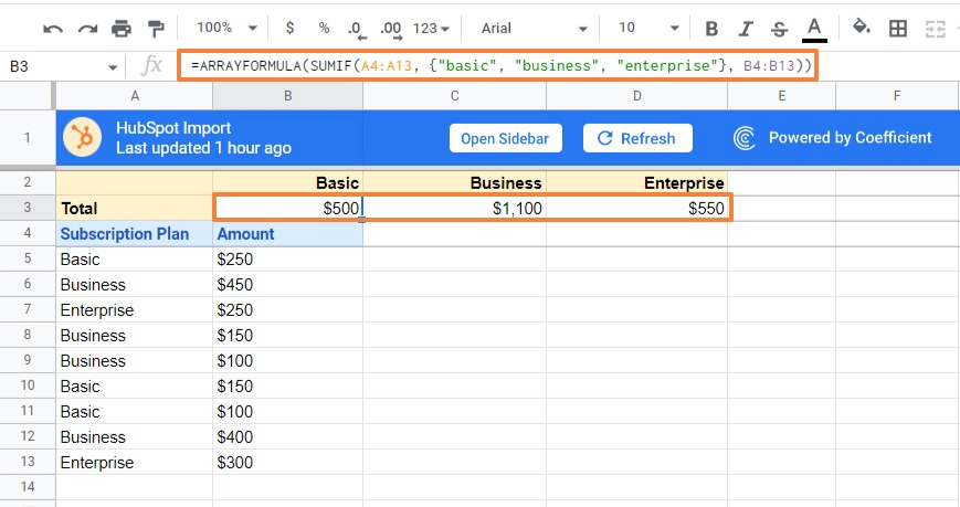
Ensure you have empty cells to the right of the cell containing the formula. Google Sheets automatically places the results into cells corresponding to the number of items in your array constant. 

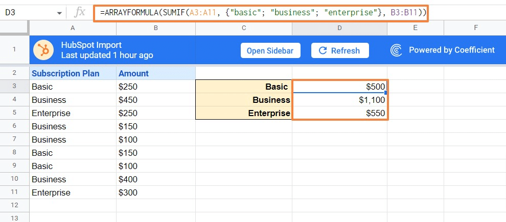
If you want to have your subtotals show in a column, make a vertical array by separating the elements with semicolons:

=ARRAYFORMULA(SUMIFS(A3:A11, {“basic”; “business”; “enterprise”}, B3:B11))

Additionally, you can use a range reference to make your formula more flexible. This way, other users in your team can type items in the predefined cells, and you won’t need to update your formula. 

For instance, the formula shown above can take this form:

=ARRAYFORMULA(SUMIFS(A3:A11, D3:D5, B3:B11))

Using SUMIFS with multiple OR criteria in different columns

You can also leverage the SUMIFS function to sum numbers with multiple sets of conditions based on the following logic:

• All conditions must be true (AND logic) in each set
• A cell is summed if any set of conditions is true (OR logic)

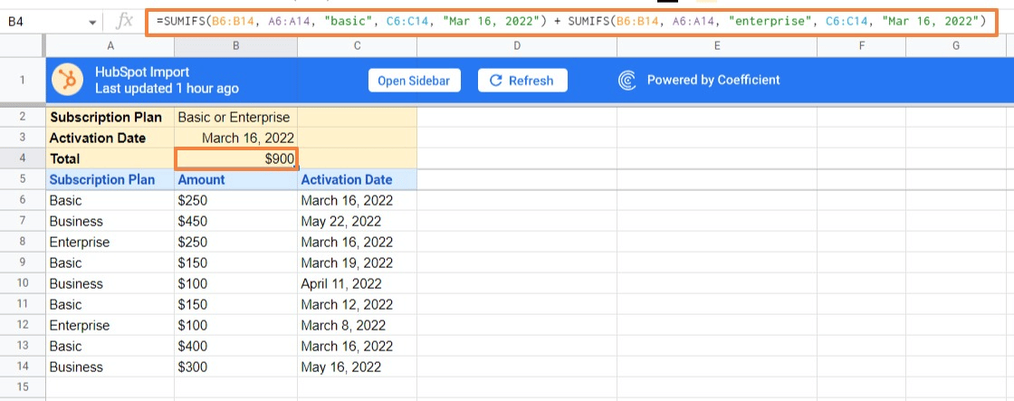
Here’s an example. Let’s sum the amount in column B if column A is either Basic or Enterprise and the activation date in column C is March 16, 2022. 

The obvious method is to take two SUMIFS formulas to add Basic and Enterprise separately, then add the results:

=SUMIFS(B6:B14, A6:A14, “basic”, C6:C14, “Mar 16, 2022”) + SUMIFS(B6:B14, A6:A14, “enterprise”, C6:C14, “Mar 16, 2022”)

But Google Sheets does not allow array constants with multiple OR conditions. Instead, you can use a slightly shorter formula featuring the SUMPRODUCT function. 

Use the formula below to sum numbers within B6:B14 based on the criteria above. 

=(SUMPRODUCT(–(C6:C14=B3), (–(ISNUMBER(MATCH(A6:A14, B2:C2, 0)))), B6:B14)) 

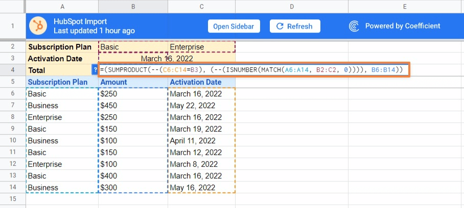
Here’s how the different parts of the formula work. 

• Determine whether an item is Basic or Enterprise: ISNUMBER(MATCH(A6:A14, B2:C2,0)). You’ll get a TRUE value if any specified criteria are met, and a FALSE value if none of the criteria are met.   

• Compare the list of dates with the target date: C6:C14=B3. Also, you can enter the date directly in the formula instead of a cell reference by using the DATE or DATEVALUE functions. For instance, use C6:C14=DATEVALUE(“March 16, 2022”) or C6:C14=DATE(March 16, 2022).

• Transform both TRUE and FALSE arrays to 1 and 0 using the double unary operator (–).  

• Provide the range to sum: B6:B14

Only the values that correspond to the specified Subscription Plan and Activation Date will get summed.   

SUMIFS function: A versatile method for summing values based on conditions

A SUMIFS function makes it easier to sum values based on predefined conditions over a range of cells. If you can master SUMIFS and its variations, you can enhance your spreadsheet capabilities and make your formulae more efficient and elegant.

Our customers typically use SUMIFS to perform more insightful analyses, while also optimizing spreadsheet performance. They implement the SUMIFS function with live data in Google Sheets via Coefficient. 

Try Coefficient for free right now!