How to Use The COUNTIF Google Sheets Function

COUNTIF in Google Sheets can count items in a cell range more efficiently than the COUNT function. COUNTIF allows you to avoid manually intensive formulae, especially when you’re analyzing large rows and columns of data.

The following guide will show you everything you need to know about the COUNTIF function in Google Sheets, including why it’s important, several easy-to-follow examples, and how to deploy the function in different scenarios. Also, watch our complete video tutorial below on how to use COUNTIF and COUNTIFS.

Video Tutorial: How to Use COUNTIF & COUNTIFS in Google Sheets

What does the COUNTIF Google Sheets function do?

The COUNTIF function in Google Sheets counts the number of cells in a cell range that meet a specified condition. The function is a practical tool when you want to know the number of times a specific criterion is met within a range of cells.

You can only test one condition using the COUNTIF function.  By default, the COUNTIF function will look for an exact match. You can also use a COUNTIF formula to assess if the values meet more complex conditions.

For example, you can test if cell values are less than, greater than, or not equal to a certain number. You can also count all the instances where a string or keyword appears as text within a cell range.

COUNTIF Function Syntax

The COUNTIF function in Google Sheets has the following syntax:

=COUNTIF(range, criterion)

range refers to the range of cells that contain the data you want to count.

criterion is the condition that must be met for a cell to be counted.

The cell range can have text strings or numbers. The criteria can use comparison or logical operators if the range of cells contains numbers, including:

• > greater than
• < less than
• >= greater than or equal to
• = equal to
• <= less than or equal to
• <> not equal to

For instance, to count the number of sales reps who closed more than 50 deals in the year’s first quarter, use >50 as your criterion. Remember to enclose operators with numbers in double-quotes.

The criterion can also be a text string in double quotes or a cell reference containing the text string. You can include wildcard characters as part of the text. For example, to count cells that contain the text string “Open,” use Open*  as the criterion.

Google Sheets COUNTIF Function: Important Considerations

Consider these critical factors about the COUNTIF function to construct superior formulae and avoid common errors.

• Numeric criterion. Numeric values with exact matches don’t require quotes.
• Conditional tests. Use logical operators to make conditional tests and enclose them in double quotes in your formula.
• Case insensitive. The COUNTIF function is case insensitive, so you’ll get the same result whether you use upper or lower cases in your formula.
• Counting blank and non-blank cells. Use empty double quotes (“”) to count blank cells within a range. Use the not-equal (“<>”) logical operator to count non-blank cells in a range.
• Reference another cell. You can contain the criterion for the COUNTIF function in a separate cell, which the formula can reference.
• Using wildcards. The Google Sheets COUNTIF function supports three wildcards: the star, question mark, and tilde.
  • The star (*) wildcard matches zero (or more) characters. It can go in your search string’s front, end, or both ends. You can also use it in reference cells.
  • The question mark (?) wildcard matches a single character. For example, if your formula is =COUNTIF(A3:A23,”A?r”), using the formula will match any string with three characters where the first and last characters are “A” and “r”.
  • The tilde (~) allows you to search for an star or question mark instead of using them as wildcards. For example, =COUNTIF(E2:E23,”No~*”) counts all the cells containing No*, and =COUNTIF(E2:E23,”No~?”) counts all cells with No?.

How to Use the COUNTIF Google Sheets Function

Let’s set up our sample dataset in Google Sheets so we can show off some examples of COUNTIF.

We’ll use Coefficient to import sales data from Salesforce into Sheets. Coefficient automatically syncs your spreadsheet with your business systems, and offers pre-built Google Sheets dashboards for popular use cases.

We’ll use the imported dataset below for our examples.

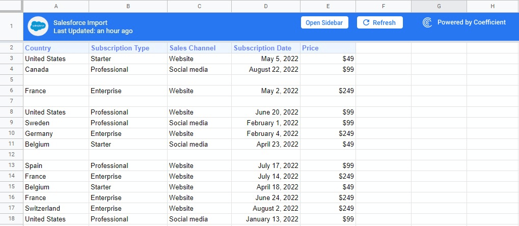
Now that we have our dataset let’s dive into some step-by-step examples of COUNTIF in Google Sheets.

Using Google Sheets COUNTIF to count cells containing certain text

As discussed, you can use a COUNTIF formula to count the number of cells within a data range that contain a specific text or numeric value.

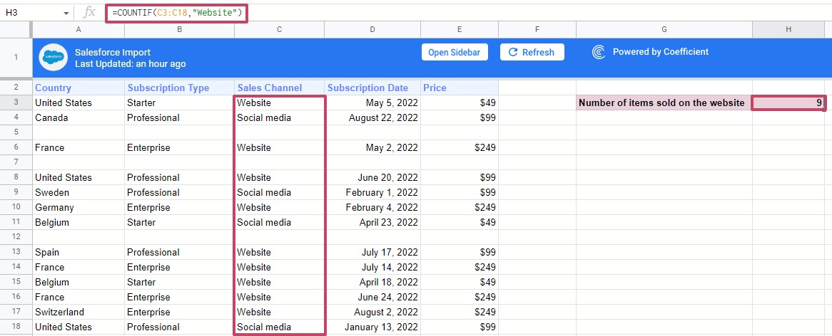
For instance, let’s say you want to find the total number of items your sales team sold via your website in our sample data set.

To do this, you’ll need to count the number of cells in column C containing “Website”.

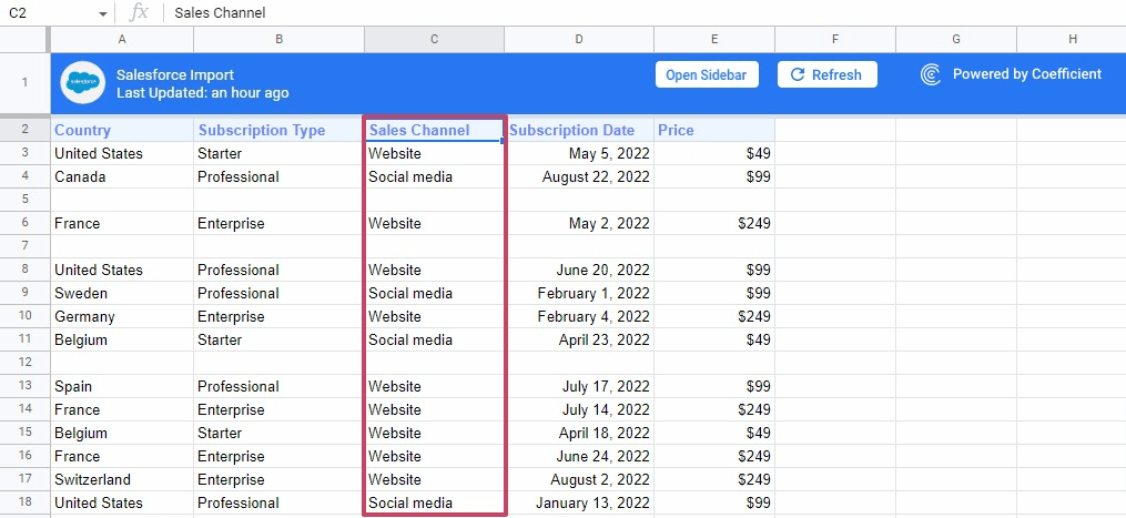
Use a COUNTIF formula to count the items in column C.

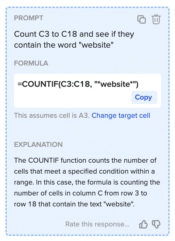
=COUNTIF(C3:C18,”Website”)

Use AI to Generate COUNTIF Formulas

You can use Coefficient’s free Formula Builder to automatically create the more basic formulas above or the advanced COUNTIF formulas below. To use Formula Builder, you need to install Coefficient. The install process takes less than a minute.

You can get started for free right from our website. 

Accept the prompts to install. Once the installation is finished, return to Extensions on the Google Sheets menu. Coefficient will be available as an add-on.

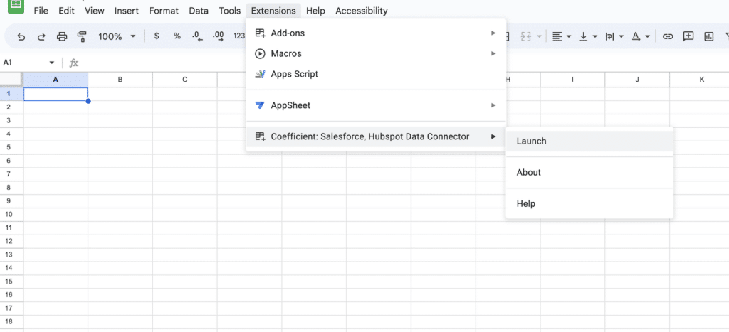
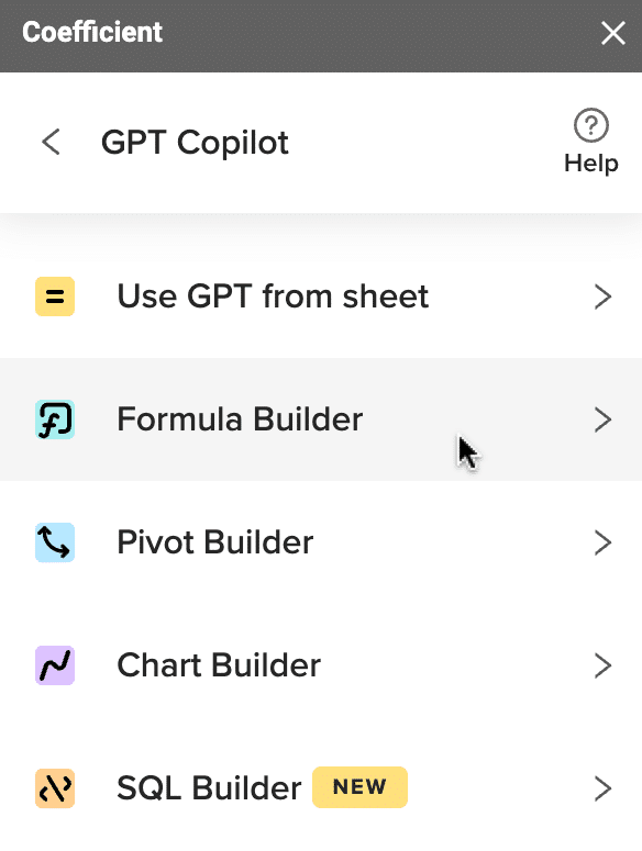
Now launch the app. Coefficient will run on the sidebar of your Google Sheet. Select GPT Copilot on the Coefficient sidebar.

Then click Formula Builder.

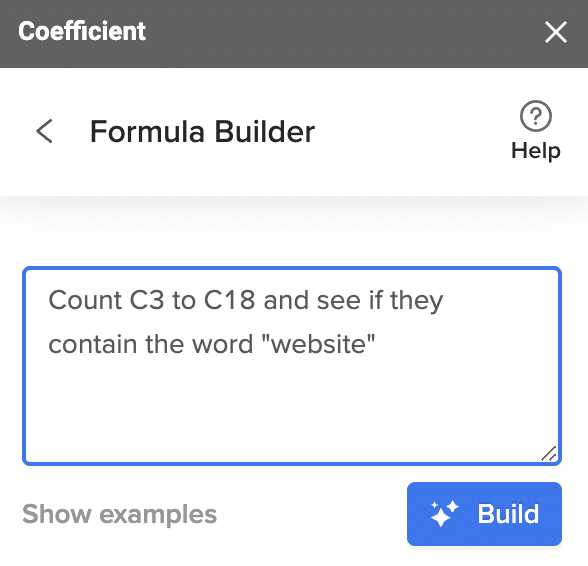
Type a description of a formula into the text box. For this example, type: Count C3 to C18 and see if they contain the word “website”.

Then press ‘Build’. Formula Builder will automatically generate the formula from the first example.

Using Google Sheets COUNTIF to count non-blank cells

You can count the number of blank and non-blank cells within your data range using the COUNTIF function.

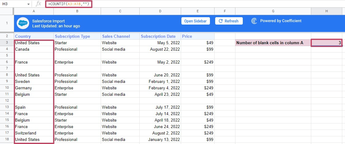
For example, if you want to count the number of blank cells in column A, use this formula:

=COUNTIF(A3:A18,””)

Use the formula below to count the number of non-blank cells in column A.

=COUNTIF(A3:A18,”<>”)

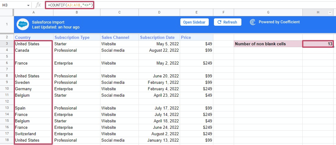
If you want to count the number of non-blank cells containing only text values, use this formula:

=COUNTIF(A3:A18,”*”)

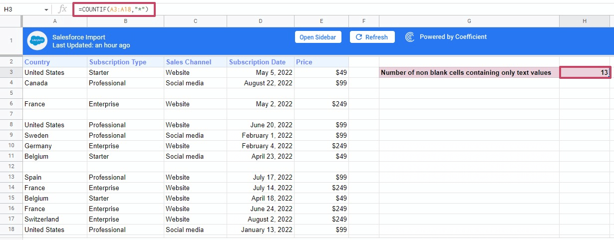
Using Google Sheets COUNTIF to count cells based on the date

Use the COUNTIF function to set certain criteria involving dates and other numeric values.

For example, to count the number of Subscription Types that started on May 2, 2022, use this formula:

=COUNTIF(D3:D18,”May 2, 2022″)

Remember to enclose the date criterion in double quotes.

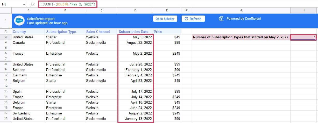
Using COUNTIF and logical expression to count cells

Suppose you want to find values less than, greater than, equal to, or not equal to a certain number, rather than exact matches.

Free AI-Powered Tools Right Within Your Spreadsheet

Supercharge your spreadsheets with GPT-powered AI tools for building formulas, charts, pivots, SQL and more. Simple prompts for automatic generation.

As an example, let’s say you want to count all the Subscriptions that started before August 22, 2022.

You can do this by combining COUNTIF with a logical criterion, as shown below.

=COUNTIF(D3:D18,”<August 22, 2022″)

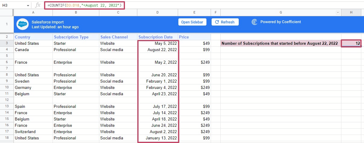
You can also use a logical criterion with numerical values. For instance, to count all the Subscriptions valued at less than $299, deploy this formula,

=COUNTIF(E3:E18,”<$299″)

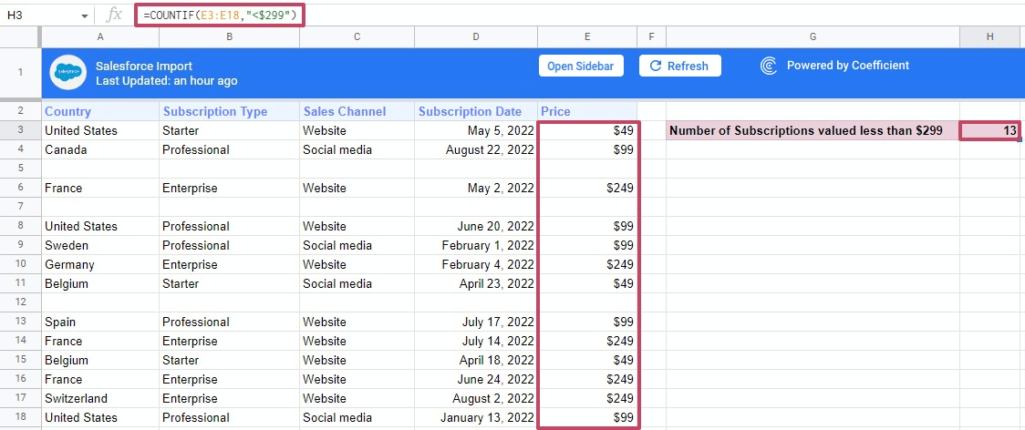
Important note: You can combine logical criteria with OR and AND functions.

Using Google Sheets COUNTIF to count all instances a keyword appears

There might be instances where you’ll need to handle data that contains variations of the same item. In the Subscription Type column below, the text of “Professional” and “Professional Plan” differs, but they should count as the same item.

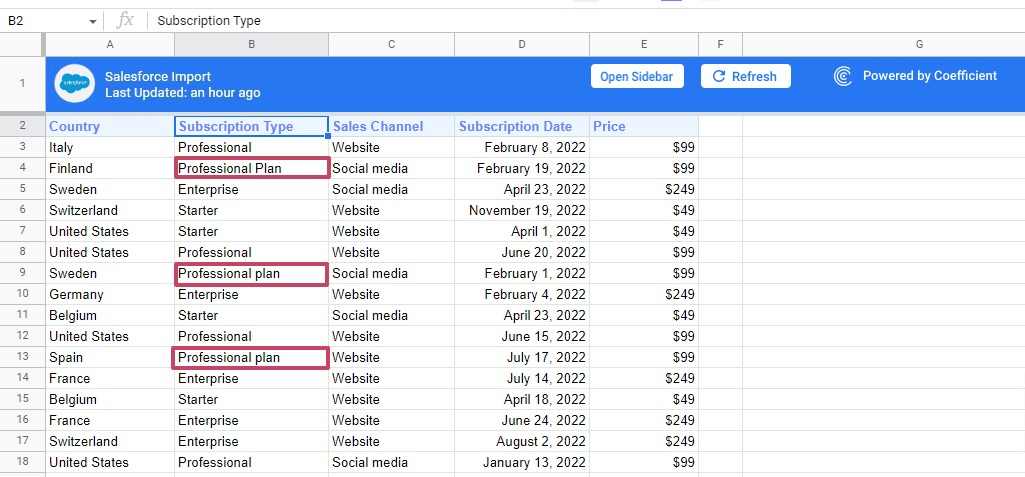
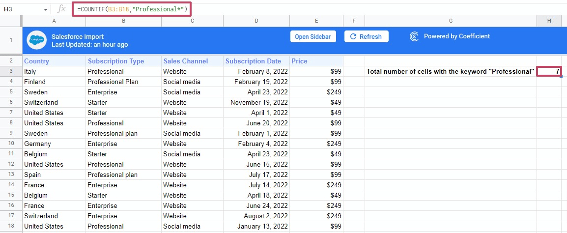
Use this formula to count the total number of cells with the keyword “Professional”:

=COUNTIF(B3:B18,”Professional*”)

How to count checkboxes or TRUE and FALSE values in a range

In order to count how many cells contain “TRUE” in a given range, use a formula like this:

=COUNTIF(Sheet1!A1:D20,TRUE)

Since TRUE and FALSE are binary values, they do not need quotation marks like normal text values. Note: When working with checkboxes in cells, those are handled the same way as TRUE and FALSE cells, meaning you can count the number of “checked” cells with the same formula above.

How to count cells in multiple Sheets using COUNTIF

The COUNTIF function works across multiple Google Sheets. For instance, say you have 18 transactions in Sheet1 and another 18 transactions in Sheet2.

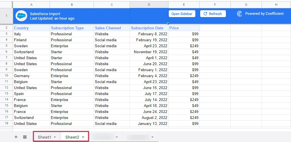
Let’s say you want to count the total number of Starter subscription plans on both Sheets.

You could use a COUNTIF function to count the cells from each Sheet separately. Then add the two like this:

=COUNTIF(Sheet1!B3:B18,”Starter”)+COUNTIF(Sheet2!B3:B18,”Starter”)

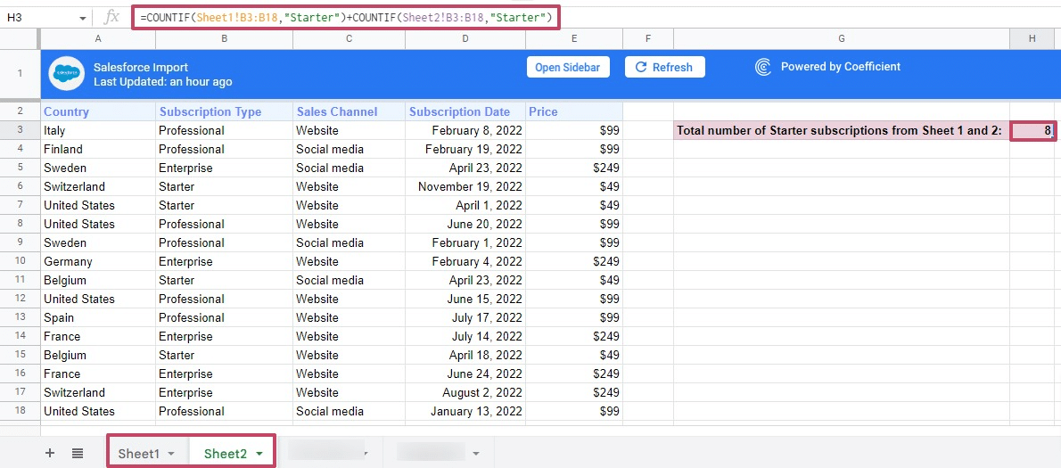
However, this method isn’t practical if you’re working with many different Sheets.

A more elegant solution is to use an array combining the “Subscription Type” list from all your Sheets into a single one with this formula:

=COUNTIF({Sheet1!B:B;Sheet2!B:B},”Starter”)

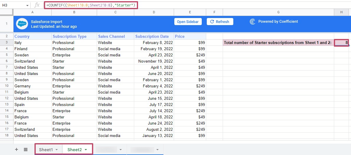
We’ll get the same results, but using an array leads to a shorter and more compact formula.

Use COUNTIFS instead of COUNTIF to filter on multiple criteria

In the example just above, if we want to count only the rows with “Website” in column C and “Professional” in column B, we could swap a COUNTIFS function into the formula:

=COUNTIFS(C3:C18,”Website”,B3:B18,”Professional”)

COUNTIFS is also very useful to count only rows that contain a value that falls between two other values, or in between two dates. For example if we wanted to only count rows with “Website” in column C and only where the Subscription Date was during the month of July 2022, we could use this:

=COUNTIFS(C3:C18,”Website”,D3:D18,”>=July 1, 2022″,D3:D18,”<August 1, 2022″)

COUNTIF function: A reliable tool that accelerates your work

The Google Sheets COUNTIF function is often the quickest way to count how many times an item appears in a defined cell range. The function’s straightforward but powerful capabilities simplify your work in Google Sheets. And you can also automate your dashboards and workflows in Google Sheets with Coefficient.

Try Coefficient for free to supercharge your spreadsheet and unlock new possibilities with your data in Google Sheets.