
This guide to IFERROR in Google Sheets will show you how to detect and contain broken formulas so they don’t disrupt your spreadsheet.
Read the following blog to learn how to use IFERROR in Google Sheets, through easy-to-follow examples and step-by-step walkthroughs.
Video Walkthrough: How to Use IFERROR in Google Sheets
What the IFERROR Function Does in Google Sheets
The IFERROR function is designed to identify and replace errors in your Google spreadsheet with preset values.
IFERROR wraps around a formula in Google Sheets, and ascertains if the formula is incapable of executing correctly.
If the formula returns any errors, the function returns a preset value that you’ve specified, or blank text. The IFERROR function is mainly used for:
- Identifying errors
- Replacing default error messages with custom messages
- Swapping error values for fallback values
- Managing arguments or parameters in an ARRAYFORMULA
IFERROR is leveraged for a wide variety of reasons, with use cases as diverse as:
- Checking if URLs match
- Sorting your data with specific conditions
- Checking title tag lengths and meta descriptions
Ultimately, IFERROR helps ensure that your spreadsheet workflows operate seamlessly, whether you’re generating monthly marketing reports or building sales dashboards in Google Sheets.
Types of Google Sheets Errors — And Why They Matter
The IFERROR function returns a specified value when a formula contains a parse error. A parse error occurs when Google Sheets can’t interpret or perform a formula operation.
In Google Sheets, parse errors are formal objects that can be leveraged by functions such as IFERROR. Parse errors can transpire due to typos, mathematical impossibilities, or any other issues that obstruct a formula.
Before you can deal with parse errors using the IFERROR function, you need to know the various error types and what they mean. Read about the common error codes that Google Sheets returns below.
The #REF Error
A #REF error in Google Sheets occurs when a formula contains an invalid reference, including:
- A missing reference
- A circular reference
- An out-of-bound cell
The #NA Error
An #N/A error in Google Sheets means that a specific value is not available. This happens when a function tries to leverage an inaccessible cell.
The error typically occurs in lookup functions, VLOOKUP. Read our ultimate guide to VLOOKUP in Google Sheets to learn more about this lookup function.
The #NAME? Error
A function usually returns a #NAME? error in Google Sheets when there are problems with a formula’s syntax.
The error could be caused by a wrong name range, spelling mistake, or the misuse of quotes within a parameter value.
The #DIV/0! Error
In Google Sheets, formulas that try to divide by zero will return the DIV/0! error. Dividing a number by zero is mathematically impossible, prompting Google Sheets to terminate the formula’s execution.
The #VALUE Error
The #VALUE error code transpires when a parameter within your formula is a type that the function does not expect.
For example, if you use a number parameter in a function that only accepts text, the function will return a #VALUE error message.
The #ERROR! Message
Google Sheets returns the #ERROR! message when it can’t determine what’s wrong with the formula. This allows Google Sheets to flag faulty formulas, even if it can’t pinpoint the specific error.
The #ERROR! message can occur when:
- An important operator is missing in the formula
- There are unequal numbers of opening and closing brackets in a formula
- There’s an equal sign at the beginning of a text that isn’t a formula
The #NUM! Error
A function returns a #NUM! error when the formula contains invalid numeric values.
For instance, this error can occur when a function returns a number too big for Google Sheets to process, or when it tries to find the square root of a negative number.
IFERROR Function Syntax
The IFERROR function’s syntax is:
IFERROR(test_value, [value_if_error])
Let’s break down how the syntax works.
- test_value is the cell reference, formula, or value the function tests for errors
- value_if_error is the value returned if test_value finds an error. It’s an optional parameter.
The IFERROR function returns test_value if it does not contain an error. If there is an error with test_value, the function returns value_if_error. If value_if_error is unspecified, the function returns a blank value.
How to Use IFERROR in Google Sheets
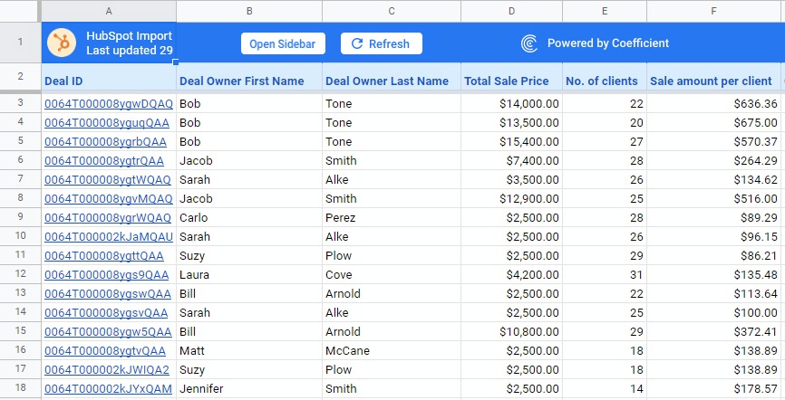
Before discussing use cases for IFERROR, let’s set up sample data to work with. We’ll use Coefficient to pull real-time data from HubSpot into Google Sheets.
For a full walkthrough on how to do this, read our blog: how to connect HubSpot to Google Sheets.
Coefficient runs as a Google Sheets add-on that lets you pull live data from your business systems into Google Sheets in seconds.
Now that we have a dataset in the spreadsheet, let’s review various examples for the IFERROR function.
Example 1: Return a Value Instead of an Error Code
The IFERROR function can return preset values instead of error codes. This is the most common use of the function.
Here’s an example. In the dataset below, the calculation returns a #DIV/0! Error, because it tries to divide by zero (cell E6).
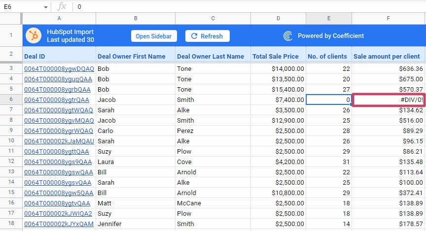
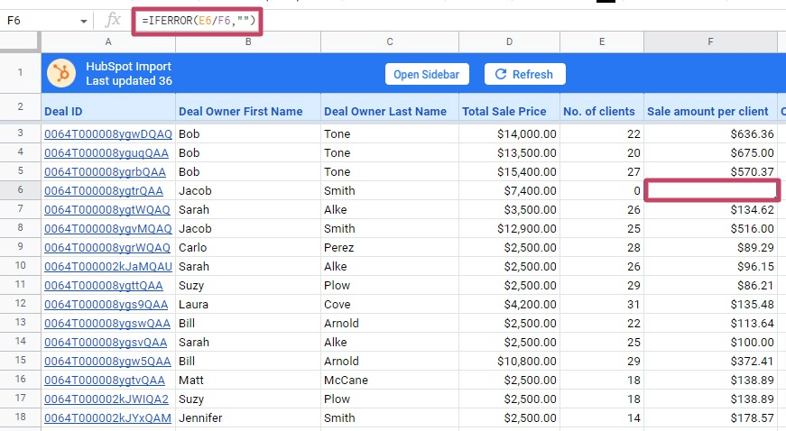
If you want to return a blank value instead of the #DIV/0! error code, use the following IFERROR formula:
=IFERROR(E6/F6,””)
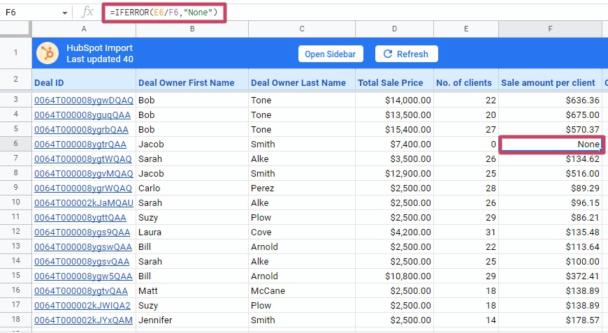
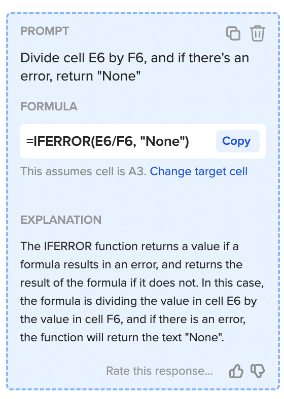
You can also use an IFERROR formula to return preset text instead of a blank cell. For instance, the formula below will return the text “None” when the calculation returns an error value.
=IFERROR(E6/F6,”None”)
AI + Google Sheets: Use Formula Builder to Automatically Generate IFERROR Formulas
You can also use Coefficient’s free Formula Builder to automatically create the formulas in this first example. To use Formula Builder, you need to install Coefficient. The install process takes less than a minute.
We’ll outline how to install Coefficient from the Google Workspace Marketplace. Or you can skip the marketplace altogether, and get started for free right from our website.
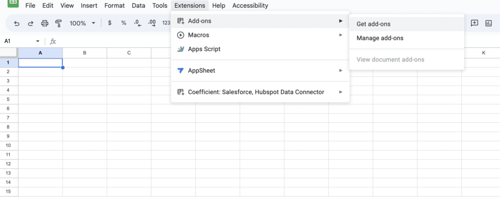
First, click Extensions from the Google Sheets menu. Choose Add-ons -> Get add-ons. This will display the Google Workspace Marketplace. Here a direct link to Coefficient’s Google Workspace Marketplace listing.
Search for “Coefficient”. Click on the Coefficient app in the search results.

Accept the prompts to install. Once the installation is finished, return to Extensions on the Google Sheets menu. Coefficient will be available as an add-on.
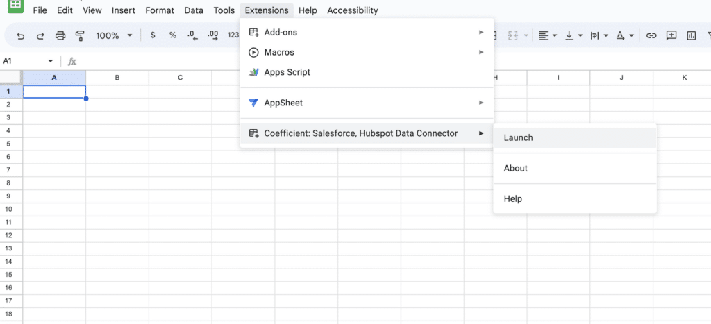
Now launch the app. Coefficient will run on the sidebar of your Google Sheet. Select GPT Copilot on the Coefficient sidebar.

Supercharge your spreadsheets with GPT-powered AI tools for building formulas, charts, pivots, SQL and more. Simple prompts for automatic generation.


Then click Formula Builder.

Type a description of a formula into the text box. For this example, type: Divide cell E6 by F6, and if there’s an error, return “None”.
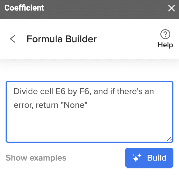
Then press ‘Build’. Formula Builder will automatically generate the formula from the first example.
Example 2: VLOOKUP Cannot Find a Lookup Value
A VLOOKUP function returns a #N/A! Error when it can’t find the lookup value. However, you can use the IFERROR function to return a preset value instead of the error message.
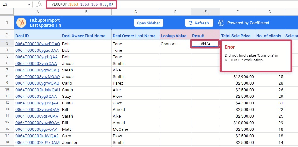
In the example below, cell E3 displays an #N/A error, since the VLOOKUP formula can’t find the lookup value in the B3:C18 cell range.
=VLOOKUP($D$3,$B$3:$C$18,2,0)
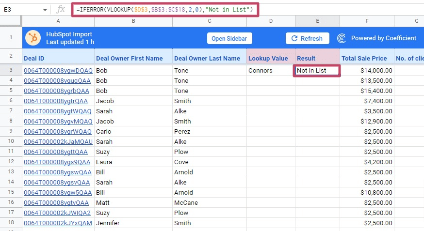
Use the formula below in cell E3 to return “Not in List” instead of the #N/A error code.
=IFERROR(VLOOKUP($D$3,$B$3:$C$18,2,0),”Not in List”)
You can also use the IFNA function instead of an IFERROR formula. If the error is #N/A, the IFNA function returns the value you’ve specified.
Example 3: Use IFERROR in ArrayFormulas
The IFERROR function is helpful when you’re using the Array Formula function in Google Sheets.
In the example below, we’ve used an array formula to quickly divide the values in column E with those in column D.
=ARRAYFORMULA(E3:E18/D3:D18)
This gives us all the results of column F in just one formula.
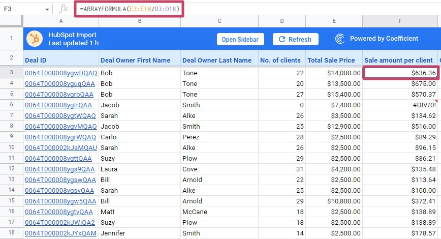
You’ll notice that the row six result (cell F6) shows a #DIV/0! error since you are trying to divide by the cell value in D6, which is zero.
Here’s the solution: wrap the Array Formula inside the IFERROR function, like this:
=IFERROR(ARRAYFORMULA(E3:E18/D3:D18))
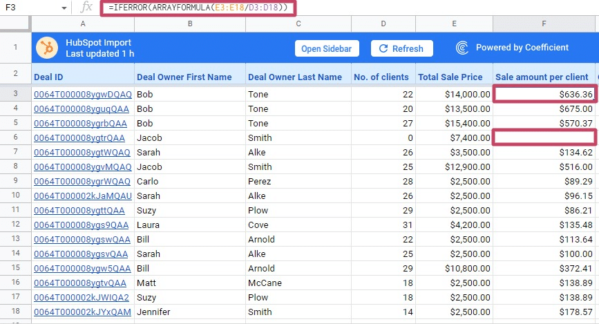
This formula applies the IFERROR function to every value within the returned array. Now you’ll see a blank cell in F6 instead of the error.
Limitations of the IFERROR function in Google Sheets
The IFERROR function is a generic solution to all formula and operations errors in Google Sheets.
The downside of the function is that it doesn’t differentiate the various error messages and treats them all the same.
Whether you get a #VALUE or #REF! error, the IFERROR function will always return the same value_if_error.
This can make troubleshooting the errors challenging for other users, since they won’t know the type of error they’re dealing with.
In the same sense, the IFERROR function can also hide errors, since spreadsheet users will only see the value_if_error specified.
Other Formulas Similar to IFERROR in Google Sheets
Besides the IFERROR function, you can use similar formulas to ensure that errors don’t disrupt your spreadsheets, including:
- IFNA: =IFNA(value, value_if_na). The IFNA function returns the first argument’s value if it’s not null and returns the second argument’s value if the first argument is null.
- IF Statement: =IF(logical_expression, value_if_true, value_if_false). The IF function returns the first argument’s value if it’s not false, and the second argument’s value if the first argument is false.
Keep Your Spreadsheets Running Smoothly with the IFERROR Function
Using IFERROR in Google Sheets is one of the most efficient ways to handle errors in your spreadsheet formulas.
The IFERROR function has limitations, but in general it’s a useful way to keep spreadsheet operations and analysis running smoothly.
And now you can combine IFERROR with live data from your company systems using Coefficient for seamless data analysis.
Try Coefficient for free now to import real-time data from Salesforce, HubSpot, and other business systems into Google Sheets.