

Click Format > Conditional formatting from the top menu to access Conditional format rules
Select the data range you want to apply the formatting rule to (e.g., E2 for Sales Price column)
Choose between Color scale option for gradient formatting or single color for basic highlighting
Configure the “Format cells if…” section with your specific formatting rules (text, date, or number conditions)
For advanced formatting, use custom formulas by selecting “Custom formula is” option
This is a complete guide to conditional formatting in Google Sheets. In this blog, you’ll learn everything you need to know about the topic.
In Google Sheets, we can apply a custom format to a cell based on its values or the values of different cells. This is called conditional formatting and it’s a potent tool to visually accentuate data and tables.
Google Sheets provides two types of conditional formatting: color scale and single color. While each operates similarly, there are key differences in how each option works.
Here’s a full overview of both types of conditional formatting in Google Sheets, based on real examples and step-by-step walkthroughs. Also, watch the tutorial below for a complete video guide on how to use conditional formatting in Sheets.
Video Tutorial: Conditional Formatting in Google Sheets (Step-by-Step Walkthrough)
Color Scale Conditional Formatting
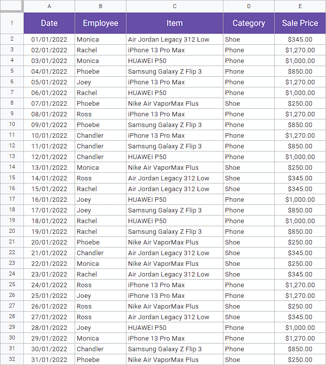
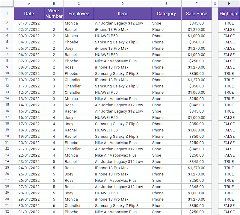
Despite the complicated sounding name, color scale conditional formatting is the simplest option to implement in Google Sheets. Let’s look at some examples of color scale, based off the following dataset:
On the top menu of Google Sheets, click Format > Conditional formatting. This will take us to Conditional format rules.
To create a conditional formatting rule, we must select the data range we want to apply the rule to. In this case, let’s choose the Sales Price (E2:E32).
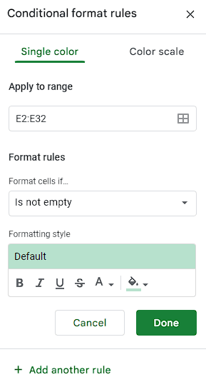
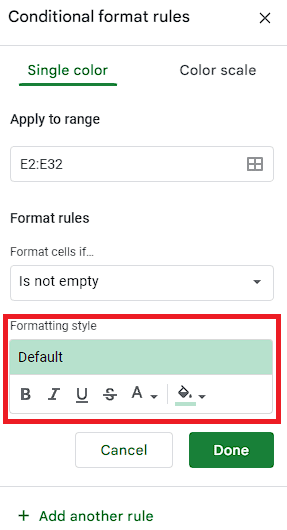
We’ll see the default conditional formatting rule: a single color (default green) applied to Is not empty (non-empty) cells.
Then click the Color scale option on the top right of the menu.
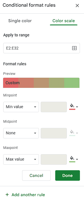
Now we’ll adjust the colors of the Minpoint and Maxpoint to create a color scale for our formatting rule.
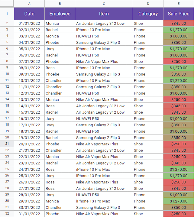
In the example above, lower sales prices will appear dark red, while higher sales prices will appear dark green.
Mid-range prices will appear in lighter shades of red and green. Click Done and our table will look like this:
We can change the Minpoint, Midpoint, and Maxpoint to flat numbers, flat percents, or percentiles. We can also set Min value and Max value properties for the conditional formatting.
Single Color Conditional Formatting
Single color conditional formatting evaluates each individual cell in the specified data range. If a cell passes the formatting rule, then the Formatting style is applied to it.
To set up single color conditional formatting, select Format > Conditional formatting. Then choose the Single color tab.
The Format cells if… section is the most important aspect of single color conditional formatting. This section offers several unique formatting rules we can deploy. Let’s go through each rule below.
Text Rules
Although Text rules suggest they can only be applied to text-formatted cells, we can actually use them on any kind of cell.
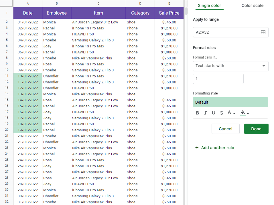
For example, let’s identify the dates in column A with days that begin in “1”.
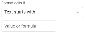
First, choose the data range A2:A32 to select the dates. Then set the Text starts with rule to “1”. This will highlight any dates in column A that start with “1”.
The result: cells A11:A20 are highlighted in light green, as specified by the Formatting style.
Here’s a complete list of all the text rules available in Google Sheets.
Conditional formatting is applied if…
- Is empty – the cell is empty or contains only spaces
- Is not empty – the cell contains any character other than spaces
-
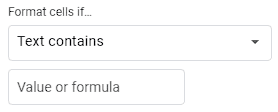
Text contains – the cell value includes the defined input
-
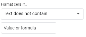
Text does not contain – the cell value does not include the defined input
-
Text starts with – the cell value starts with the defined input
-
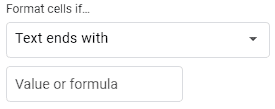
Text ends with – the cell value ends with the defined input
-
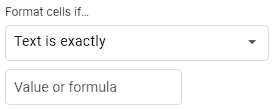
Text is exactly – the cell value exactly matches the defined input
Date Rules
Date rules are another key rule set for conditional formatting in Google Sheets. There are three types of date rules in Google spreadsheets. For Date rules, we recommend using the DATE function to input dates:
=DATE(year, month, day)
This makes entering dates more seamless. For the dataset below, let’s apply conditional formatting to the date “11/01/2022”.
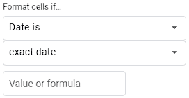
Select A2:A32 at the data range. Choose the Date is rule and Exact date under the Format cells if… section. Use the DATE function to enter the specified date (11/01/2022) into the input box.
=DATE(2022, 1, 11)

The result: conditional formatting is applied to the date 11/01/2022 in the dataset.
We leveraged the exact date filter in this example. But there are several other filters we can use, including:

Here are the other available Date rules for conditional formatting in Google Sheets.
Conditional formatting is applied if…
- Date is – the cell date value exactly matches the defined date
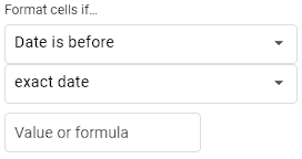
- Date is before – the cell date value is smaller than the defined date
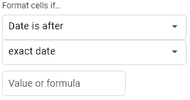
- Date is after – the cell date value is greater than the defined date
Number Rules
Number rules allow you to apply conditional formatting based on mathematical comparisons and ranges, such as greater than, less than, or in between.
Let’s say in the dataset below we want to format dates that fall between a certain date range: January 15th and January 26th.
Open Conditional format rules. Choose the Date column as the data range (A2:A32). Now, under Format rules, set the following parameters:
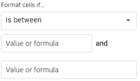
Format cells if…
Is between
=DATE(2022, 1, 15)
and
=DATE(2022, 1, 26)
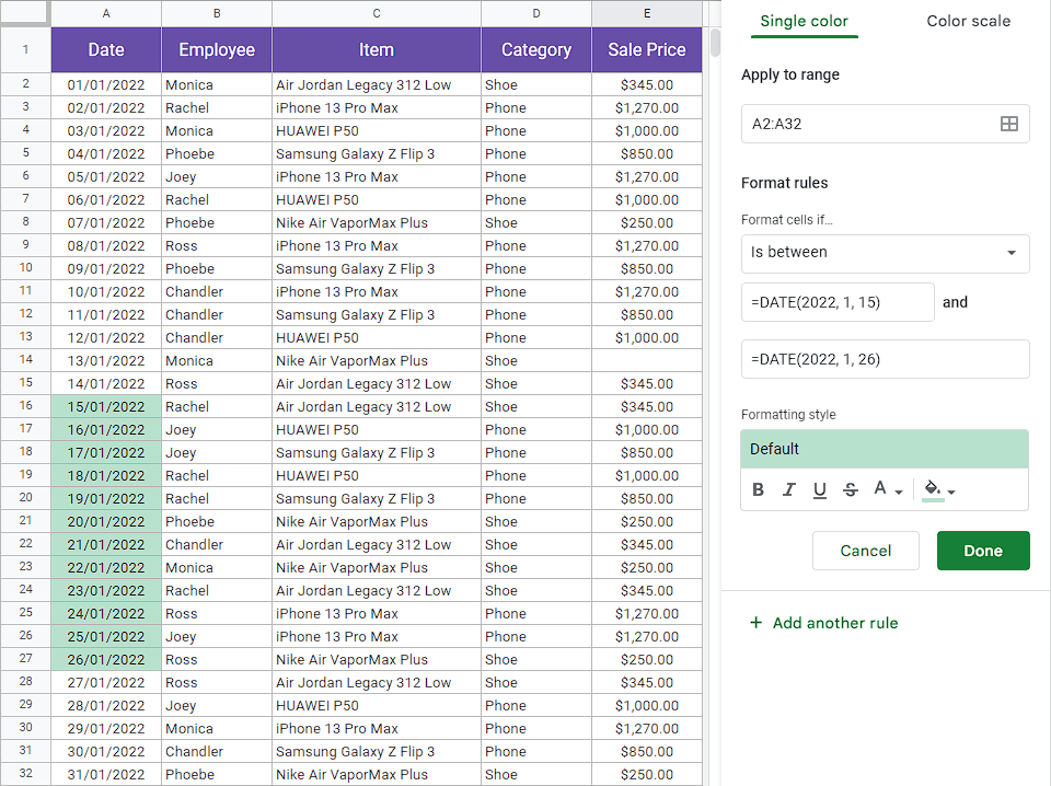
This is what the result looks like: the dates within the range turn light green. Notice that the date range is inclusive (includes both the min and max dates).
Now let’s review all the number rules available in Google Sheets.
Conditional formatting is applied if…
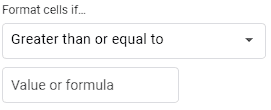
- Greater than – the cell value is greater than the defined input
- Greater than or equal to – the cell value is greater than or equal to the defined input
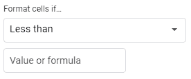
- Less than – the cell value is less than the defined input
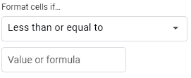
- Less than or equal to – the cell value is less than or equal to the defined input
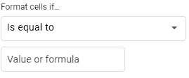
- Is equal to – the cell value is exactly equal to the defined input
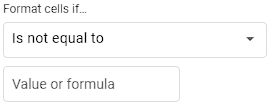
- Is not equal to – the cell value is not exactly equal to the defined input
- Is between – the cell value is between the two defined inputs (inclusive on both ends)
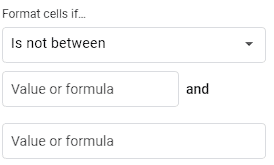
- Is not between – the cell value is not between the two defined inputs (inclusive on both ends):
Custom Formula
Conditional formatting is most powerful when it is determined by a custom formula.
To set a custom formula, launch Conditional format rules the same way as always, by clicking Format > Conditional formatting.
Under Format cells if…, select Custom formula is.
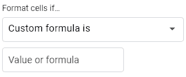
We’ll start with a simple example. Let’s say we want to highlight the rows where Ross sold an item. The formula we’ll input is:
=$B2=“Ross”

Supercharge your spreadsheets with GPT-powered AI tools for building formulas, charts, pivots, SQL and more. Simple prompts for automatic generation.

We’ll use the absolute reference symbol ($) to freeze the column we’re checking (“Employee” – column B). Conditional formatting is only activated when the value in column B = “Ross”.
And with the data range set at A2:E32, the custom formula will apply conditional formatting rules to the associated rows.
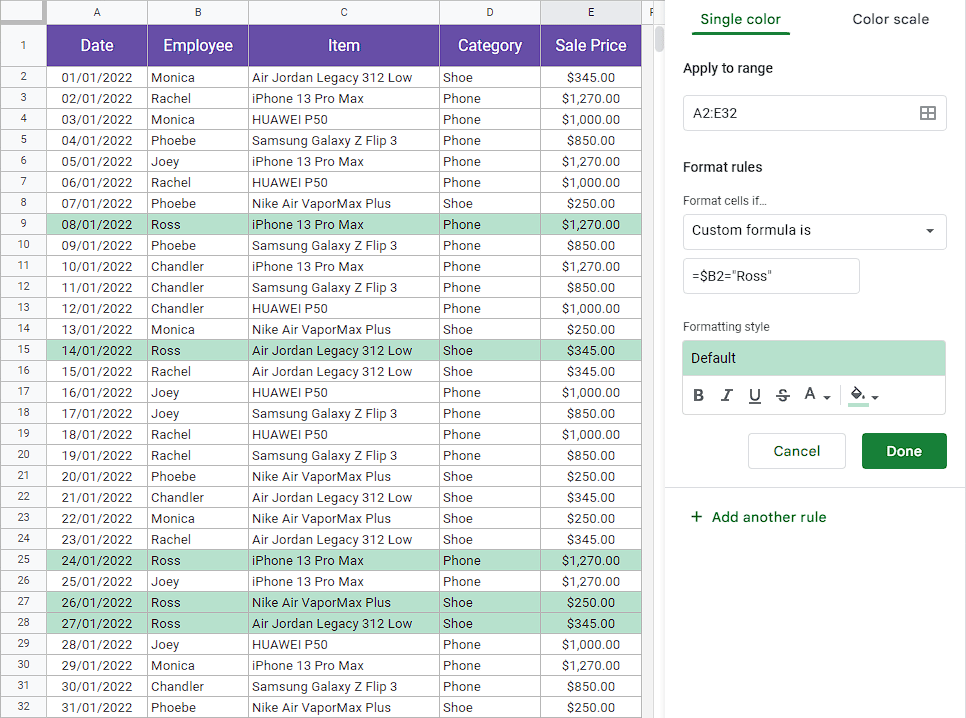
The result: all rows linked to Ross are highlighted in light green.
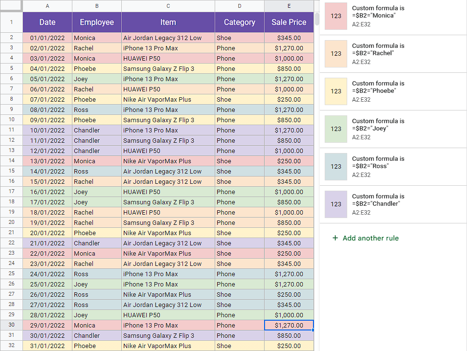
Now let’s say we want to assign a different color to each row depending on the associated employee.
Navigate to Conditional format rules and select Custom formula is under Format cells if… Enter the formula from the last example:
=$B2=“Ross”
Choose a unique color under Formatting style and press Done.
Now create the same conditional formatting rule for each listed employee.
=$B2=“Monica”
=$B2=“Rachel”
=$B2=“Phoebe”
=$B2=“Joey”
=$B2=“Chandler”
For each rule, make sure to select a unique color palette under the Formatting style section. You can see the result below: each row associated with the employee is highlighted in a distinguishable color.
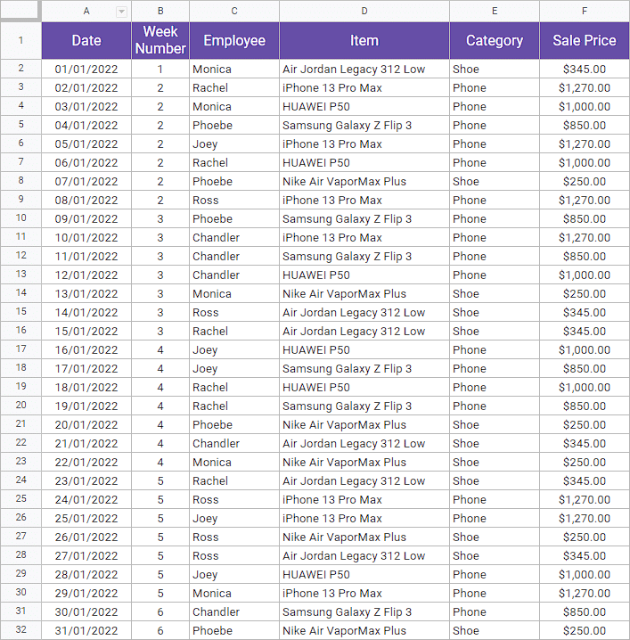
Now we can try a more advanced example. Let’s group sales based on the week they were made.
First, to make the process easier, add a Week Number column to our table, using a WEEKNUM formula:
Then add a helper column (column H) with the following formula:
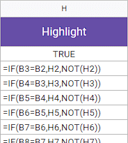
Column H should continue all the way down to H32. This returns a TRUE or FALSE value based on whether or not the week number in the current row matches the week number from the previous row.
Now let’s define the actual conditional formatting rule. Set Custom formula is to:
=$H2
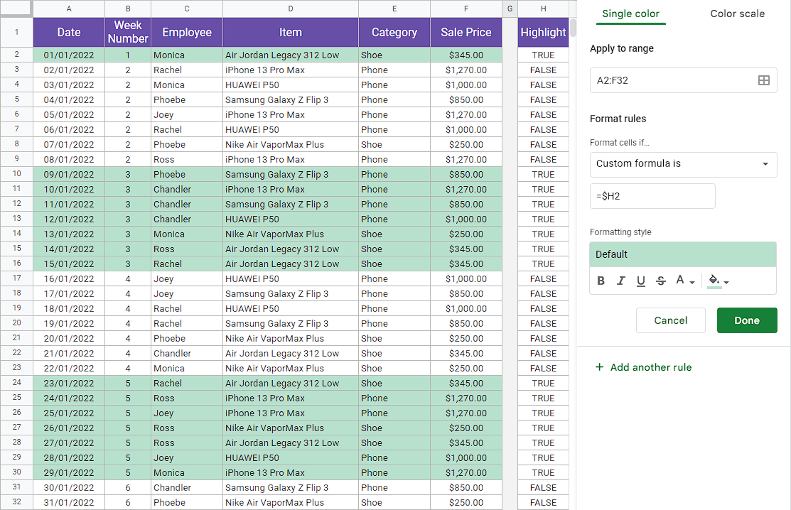
The custom formula groups sales by week in either white or light green. This makes it much easier to grasp sales by week across the month of January 2022.
Use AI to Write Formulas for Conditional Formatting
As you can see, there are quite a few you can use conditional formatting within Google Sheets. You may be a little overwhelmed, but you don’t have to go at it alone.
You can use Coefficient’s free GPT Copilot to automatically generate any spreadsheet formula, pivot, or chart, including your conditional formatting formulas. To use GPT Copilot, you need to install Coefficient. The install process takes less than a minute.
First, you’ll get started for free by simply submitted your email.
Follow along with the prompts to install. Once the installation is finished, return to Extensions on the Google Sheets menu. Coefficient will be available as an add-on.

Now launch the app. Coefficient will run on the sidebar of your Google Sheet. Select GPT Copilot on the Coefficient sidebar.

Then click Formula Builder.

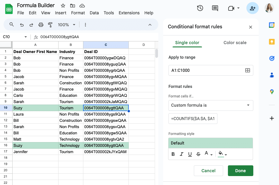
Type a description of a formula into the text box. Let’s take an example where we’re looking to highlight deals if the deal owner’s name and deal ID are both the same on multiple rows.
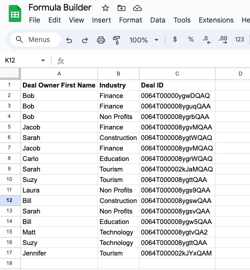
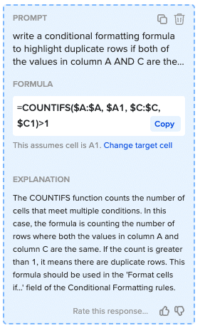
Let’s type: Write a conditional formatting formula to highlight duplicate rows if both of the values in column A AND C are the same in both rows in sheet11.

Then press ‘Build’. Formula Builder will automatically generate the formula from the first example.
Simply open up Conditional Formatting in the Format dropdown, add a new rule, select Custom Formula and paste your conditional formatting formula.
Google Sheets Conditional Formatting: Make Your Data Come Alive
Conditional formatting in Google Sheets allows you to highlight data and trends in your spreadsheet. From color scale distributions, to advanced custom formulas, conditional formatting visualizes insights in a way that makes it easier for you and your team to analyze Google spreadsheet data.
Harness Coefficient to pull real-time data from your business system into Google Sheets for free. Try Coefficient now to improve data analysis and accentuate the power of conditional formatting in your spreadsheet.