How to Use the Google Sheets QUERY Function

The Google Sheets QUERY function is often described as the most robust function in Sheets. The QUERY function combines the capabilities of many other functions in Google Sheets, including FILTERs, AVERAGEs, SUMs, and more. The function essentially allows you to run SQL-like queries against data tables in Sheets.

Here’s the ultimate guide to the Google Sheets QUERY function. Read on to learn what the Google Sheets QUERY function is, why it’s important, and examples of how to use the function in Sheets.   

What is the Google Sheets QUERY Function? 

The Google Sheets QUERY function empowers you to execute queries written in an SQL-like language called Google Visualization API Query Language in Google Sheets. These queries allow you perform database-type searching in Google Sheets, so you can find, filter, and format data with maximum versatility. 

Specifically, the function allows you to apply a query to a Google Sheets data table. This enables you to extract data subsets from the main dataset. You can think of a query as a combination between a filter and a pivot table. The QUERY function helps you inspect areas of interest within your data to gain better and deeper insights.

QUERY Function: Benefits & Advantages

Using the Google Sheets QUERY function has several benefits, including the following. 

• QUERY datasets can update in real time, allowing you to refresh your Google spreadsheets on the fly. 

• You can also reference the QUERY results for your graphs and tables and use them in other Google apps such as Google Slides or Docs. 

• Updating your QUERY datasets in your spreadsheets will update the corresponding data across the Google apps seamlessly and without error.   

• By using the QUERY function, you can import specific rows and columns based on your selected conditions and criteria. 

• The QUERY function saves you from writing individual formulas for each column, so you can avoid manually copying and pasting, or spawning errors. 

• After writing QUERY functions for specific datasets once, you can use them repeatedly and tweak them accordingly. 

In our work with teams from all over the world, these are some of the most common benefits we’ve seen for the QUERY function, though others certainly exist.

QUERY Function Syntax

The QUERY function syntax generally looks like this:

=QUERY(data, query_string, [headers])

Below is the breakdown of the three arguments:

• data – This is the range of cells (the data table) you want to analyze.
• query_string – This contains the query you want to run. 
• headers – This refers to the number of header rows in your data (with optional parameters).

Let’s take a look at a sample QUERY function:

=QUERY(A2:D345,"SELECT C, E",2)

In this example, the data range is A2:D345. 

The query_string (or query statement) is the string enclosed in quotes. It selects columns C and E from the data in this case.  

The number 2 tells the function that the original dataset contains two header rows. The argument is optional, so Google Sheets will automatically determine it if you omit it.   

Essentially, the function reads the given query in the query_string and applies it to the data. Then, it returns the resulting table acquired after the query runs. 

Below are the typical components of a query_string. 

Clauses

Clauses are parts of a query that let you filter the given data. 

Some clauses allow you to customize how you want to query your data. For instance, using the SELECT clause lets you choose specific subsets of columns from your dataset. 

On the other hand, the WHERE clause filters the selected columns based on a condition to supplement the SELECT clause. 

Aggregate Functions

An aggregate function performs calculations on values. 

Generally, aggregate functions perform the calculation then return a single value. 

Aggregate functions examples include:

• COUNT – This counts the number of rows in a column (or a subset of a column). 
• SUM – The SUM function adds all the values in the given column.
• MIN – This finds the lowest value within a column (or a subset of a column).
• MAX – The MAX function finds the highest value in a column.
• AVG – This calculates the average values in a column.    

Aggregate functions must be used together with the GROUP BY clause, or you will get an error. Also, all the aggregate functions ignore NULL values (except for the COUNT function). 

Arithmetic Operations

Arithmetic operations are essentially basic expressions consisting of a constant, variable (or scalar function) and operators such as subtraction(-), addition(+), division(/), multiplication (*), and modulus (%). 

You can use the operators to select data from your main dataset to perform mathematical operations. 

Arithmetic operations can also include comparison operators such as >, <, =, <=, >=.  

What to Consider Before Running a QUERY Function 

Below are a few tips to help ensure your QUERY function runs properly and without any issues. 

• You can write in upper or lower case (e.g., select or SELECT) since the keywords aren’t case sensitive. 
• But use column letters in uppercase, or you’ll receive errors. 
• While you don’t need to use all these keywords, ensure they appear in this order when you do: SELECT, WHERE, GROUP BY, ORDER BY, LIMIT, and LABEL. 

Follow the examples below to learn how to use the Google Sheets QUERY function. 

How to Use the Google Sheets QUERY Function

VIDEO: Step-by-Step Guide to QUERY Function in Google Sheets

Let’s assume our starting data looks like this: 

We’ll use a named range to identify the data. It makes it cleaner and easier to use in the QUERY function. 

Select your data range and navigate to the top menu to create named ranges. Select Data > Named ranges. 

A side pane will appear on the right side of your Google spreadsheet. Input a name for your data table for easy reference. 

Now we can start leveraging the QUERY function in Google Sheets. 

SELECT Specific Columns 

First, retrieve specific columns from your table with a Query function. Select a cell on the right side of the table (cell F1 in this example) and type in this QUERY function:

=QUERY(countries,"SELECT A, B",1)

A and B refer to the original table’s column references in the QUERY select statement. 

We want to select columns A and B, so your output table should retrieve and display the Rank and Country columns.  

Voila. You’ve just performed your first query. 

Use AI to Automatically Generate QUERY Formulas

You can also use Coefficient’s free Formula Builder to automatically create the formulas in this first example. To use Formula Builder, you need to install Coefficient. The install process takes less than a minute.

First, you’ll get started for free by simply submitted your email.

Follow along with the prompts to install. Once the installation is finished, return to Extensions on the Google Sheets menu. Coefficient will be available as an add-on.

Search for “Coefficient”. Click on the Coefficient app in the search results.

Accept the prompts to install. Once the installation is finished, return to Extensions on the Google Sheets menu. Coefficient will be available as an add-on.

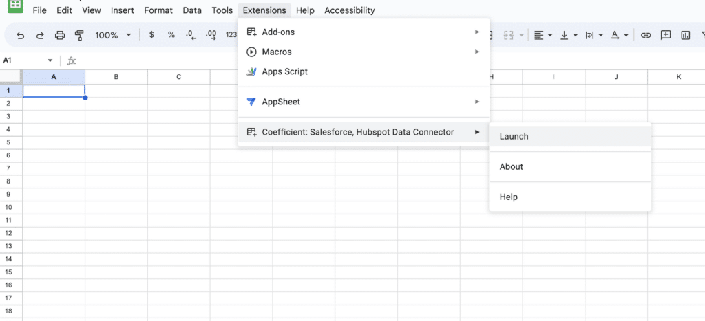
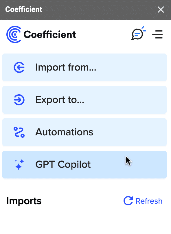
Now launch the app. Coefficient will run on the sidebar of your Google Sheet. Select GPT Copilot on the Coefficient sidebar.

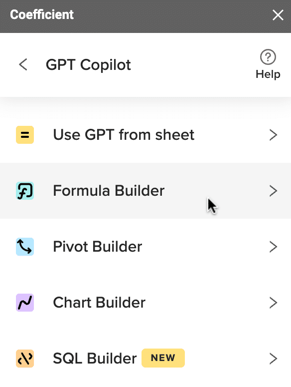
Then click Formula Builder.

Type a description of a formula into the text box. For this example, type: Run a query on data table named “countries” that outputs column A and B.

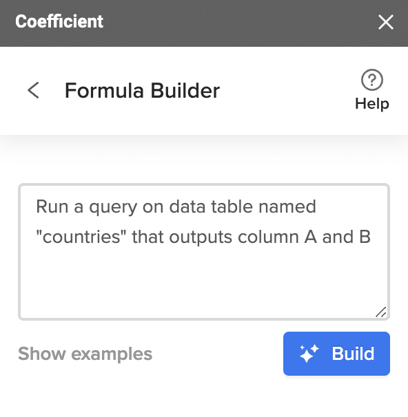
Then press ‘Build’. Formula Builder will automatically generate the formula from the first example.

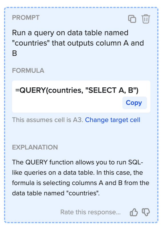
Simply paste your Google Sheets query formula in the desired cell.

SELECT All 

Use the SELECT * statement to retrieve all the columns from the data table. 

Select a cell on the right side of the table (cell F1 in this example). Input the QUERY function using the named range notation:

=QUERY(countries,"SELECT *",1)

If you’re not using Named ranges, your formula will look like this instead:

=QUERY(A1:D234,"SELECT *",1)

We’ll use the named range “countries” for the rest of the queries in this guide, but you can use the regular range reference if you want. 

Hit Enter after typing in the Query. You should see the output table. The output from the query is the entire table since SELECT * retrieves all the columns in the countries table.

WHERE Keyword

Use the WHERE keyword in your QUERY function to specify a condition that must be satisfied to filter your data.

Modify the Google Sheets QUERY function we used earlier to select the countries with a population greater than, let’s say, 10 million. 

The Query function should look like this:

=QUERY(countries,"SELECT B, D WHERE D > 10000000",1) 

The WHERE keyword comes after SELECT.  Your output table should look like this. 

Let’s do another one. 

We’ll use the WHERE keyword to specify Asian countries only in this example.

Modify your formula to this:

=QUERY(countries,"SELECT B, C, D WHERE C = 'Asia' ",1)

Unlike the numeric example earlier, you need to enclose the word Asia in single quotes within the query formula, or you’ll get an error.  

Your output table should retrieve all the specific countries in Asia. 

ORDER BY Keyword

You can use the ORDER BY keyword to sort data with your QUERY function. Specify the column (or columns) to order. This will sort your data in descending or ascending order. The ORDER BY keyword comes after SELECT and WHERE. 

 We’ll sort the data by population (from largest to smallest) in the following example. 

Insert the WHERE keyword into the old query formula. Then add the ORDER BY keyword and specify a descending direction using DESC (descending). 

=QUERY(countries,"SELECT B, C, D ORDER BY D DESC",1)

Your output table should look like this:

If you want to sort your data by country in ascending order, modify your formula to this:

=QUERY(countries,"SELECT B, C, D ORDER BY B ASC",1)

The resulting output table should display the countries in ascending order (smallest to largest population). 

LIMIT Keyword

If you want to restrict the number of results returned from your data, use the LIMIT keyword in your QUERY function. 

Place the LIMIT keyword after SELECT, WHERE, and ORDER BY. 

For instance, if we want to return only the first 15 results from our data, our formula should be:

=QUERY(countries,"SELECT B, C, D ORDER BY D ASC LIMIT 15",1)

Your data output table will look like this. 

Arithmetic Functions

You can perform standard mathematical operations on numeric columns using the QUERY function in Google Sheets.

As an example, let’s determine the percentage of the total world population that each country accounts for. 

Divide the population column by the total world population (7,162,119,434). Then, multiply the amount by 100 to calculate the percentages. 

This is what the calculation looks like as a QUERY formula: 

=QUERY(countries,"SELECT B, C, (D / 7162119434) * 100",1)

The third column in your output table should show the corresponding percentages for each country. You can format the output column to display the numbers up to two decimal places.  

LABEL Keyword

Rename your column headings easily using a LABEL keyword in your QUERY function. Place the LABEL keyword after the query statement. 

For instance, you can change the header of the output column (the third column) in the table where we retrieved the population percentages. 

Modify your formula to this: 

=QUERY(countries,"SELECT B, C, (D / 7162119434) * 100 LABEL (D / 7162119434) * 100 'Percentage'",1)

The output column heading now shows Percentage. 

Aggregation Functions

Besides calculations, you can use other functions in a QUERY, including average, min, and max. 

In this example, let’s calculate the max, min, and average populations in the “countries” dataset using these aggregate functions in your query.  

=QUERY(countries,"SELECT min(D), max(D), avg(D)",1)

The Query function returns the original dataset’s min, max, and average populations, so our output should look something like this. 

GROUP BY Keyword

You can use the GROUP BY keyword with aggregate functions to summarize your data into groups (similar to how a Pivot table does). 

We’ll summarize the data by continent and count the number of countries (per continent). 

Tweak the query formula and include a GROUP BY keyword. Also, use the COUNT aggregate function to count the number of countries.  

=QUERY(countries,"SELECT C, count(B) GROUP BY C",1)

Ensure that each column in the SELECT statement is aggregated (min, max, or counted) or appears after the GROUP BY keyword.  

The output for your QUERY function now appears as:

Let’s go over a more complex example. This time, we’ll incorporate multiple types of keywords. 

Tweak the formula to read: 

=QUERY(countries,"SELECT C, count(B), min(D), max(D), avg(D) GROUP BY C ORDER BY avg(D) DESC LIMIT 5",1)

Let’s break down the Query function into lines to make it easier to understand.   

=QUERY(countries,

"SELECT C, count(B), min(D), max(D), avg(D)

GROUP BY C

ORDER BY avg(D) DESC

LIMIT 5",1)

The QUERY function summarizes the data for each continent, sorts it from the highest to the lowest average population, and limits the results to the top five.  

Other keywords you can use in your Google Sheets Query function include OFFSET, OPTIONS, FORMAT, and PIVOT. 

You can also use other functions to add a total row, including using dates as filters in your QUERY formulas. 

Coefficient Simplifies & Streamlines Queries in Google Sheets

The Google Sheets QUERY function is a robust tool, but stale data, manual data updates, and other common spreadsheet limitations can dilute the power of the function. However, new solutions such as Coefficient are erasing these shortcomings. Coefficient is a free Google Sheets add-on that can simplify and streamline querying data in your spreadsheet.  

Coefficient automatically syncs Google Sheets with your business systems. Now you can connect live data from any system to your spreadsheet in seconds, including HubSpot, Salesforce, Jira, Snowflake, Google Analytics, MySQL, APIs, data warehouses, and databases. These connected spreadsheets enable your QUERY functions in Google Sheets to leverage real-time data at all times.  

Coefficient also allows you to run queries in SQL, SOQL, and other query languages against your systems directly from Google Sheets. And with a data inline previewer, Coefficient enables you to query and customize data tables through a no-code, graphical UI. Coefficient helps make the often complex undertaking of querying data easier, whether you want to dive into SQL, or use a point-and-click substitute.       

Google Sheets QUERY Function: The Most Powerful Tool

The QUERY function brings the power of database-style lookups to Google Sheets. Now you can combine the capabilities of some of the most incisive functions in Sheets under a single umbrella. And by adding a solution such as Coefficient, you can unlock the full potential of the Google Sheets QUERY function with AI-powered formulas, connected spreadsheets, real-time data, and more versatile queries.