Excel Lock Cells: Comprehensive Guide to Protect Your Data (2024)

Locking cells in Excel prevents accidental changes, safeguards formulas, and maintains data integrity. This guide covers everything from basic protection to advanced techniques.

How to Lock Specific Cells in Excel

Protecting individual cells is crucial for maintaining data accuracy while allowing collaboration. Here’s how to do it:

Step 1: Select the cells you want to lock.

• Open your Excel spreadsheet.
• Click and drag to highlight the cells you wish to protect.
• For non-adjacent cells, hold Ctrl while clicking each cell.

Step 2: Access the Format Cells window.

• Right-click on the selected cells.
• Choose “Format Cells” from the context menu.

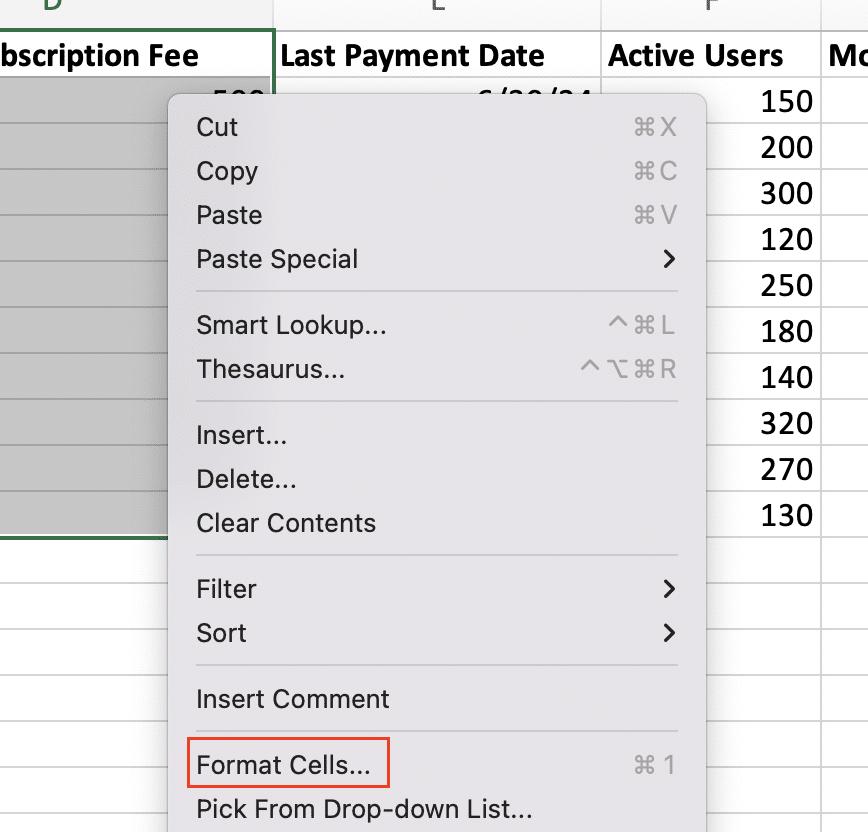
• Alternatively, use the keyboard shortcut Ctrl + 1.

Step 3: Enable the Locked option in the Protection tab.

• In the Format Cells window, click on the “Protection” tab.

• Check the box next to “Locked“.

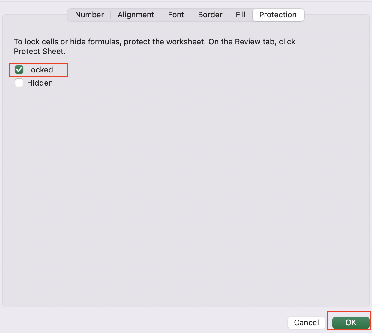
• Click “OK” to apply the setting.

Step 4: Protect the worksheet to activate cell locking.

• Go to the “Review” tab on the Excel ribbon.
• Click “Protect Sheet“.

• In the dialog box, check any option to activate cell locking.

• Optionally, set a password for additional security.

• Click “OK” to finalize protection.

Remember, locking cells only takes effect when the worksheet is protected. Always test your protection settings to ensure they work as intended.

Locking Entire Columns or Rows

Sometimes, you need to protect larger sections of your spreadsheet. Here’s how to lock entire columns or rows:

Step 1: Select the columns or rows.

• For columns: Click the letter at the top of the column.
• For rows: Click the number on the left side of the row.
• To select multiple, click and drag or hold Ctrl while clicking.

Step 2: Lock the selected columns or rows.

• Right-click on the selected area.
• Choose “Format Cells“.

• Go to the “Protection” tab.

• Check the “Locked” box and click “OK“.

Step 3: Protect the worksheet.

• Follow the same steps as in the previous section to protect the sheet.

This approach is useful when you have consistent data types or formulas across entire columns or rows. For example, you might lock a column containing employee IDs or a row with complex calculations.

Creating Editable Areas in a Protected Sheet

Sometimes you want a mix of protected and editable cells. Here’s how to achieve this:

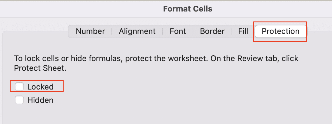
Step 1: Unlock specific cells within a protected sheet.

• Select all cells in the worksheet (Ctrl + A).
• Right-click and choose “Format Cells“.

• In the “Protection” tab, uncheck “Locked” and click “OK“.

Step 2: Lock the cells you want to protect.

• Select the cells you want to lock.
• Repeat the process to lock these specific cells.

Step 3: Protect the worksheet.

• Go to “Review” > “Protect Sheet“

.

• Set your desired options and password.

This mixed protection approach is ideal for templates where users need to input data in specific areas while other parts remain protected. For instance, in a budget template, you might leave expense input cells editable while protecting formulas and totals.

Locking Cells with Formulas

Protecting formulas is crucial to maintain the integrity of your spreadsheet calculations. Here’s how to do it:

Step 1: Identify cells containing formulas.

• Go to the “Home” tab.

• In the “Editing” group, click “Find & Select“.

• Choose “Formulas” to highlight all formula cells.

Step 2: Lock the formula cells.

• With the formula cells selected, right-click and choose “Format Cells“.

• In the “Protection” tab, ensure “Locked” is checked.

• Click “OK” to apply.

Step 3: Protect the worksheet.

• Follow the standard steps to protect the sheet.

Step 4: Test the protection.

• Try to edit a cell containing a formula.
• You should receive an error message indicating the cell is protected.

This method ensures that users can’t accidentally overwrite or modify your carefully crafted formulas, maintaining the accuracy of your spreadsheet’s calculations.

Using Password Protection for Locked Cells

Adding password protection provides an extra layer of security for your locked cells. Here’s how to implement it:

Step 1: Protect the worksheet with a password.

• Go to “Review” > “Protect Sheet“.

• Enter a strong, memorable password in the dialog box.

• Confirm the password and click “OK“.

Step 2: Set a strong, memorable password.

• Use a combination of uppercase and lowercase letters, numbers, and symbols.
• Aim for at least 12 characters.
• Consider using a passphrase for easier recall.

Step 3: Manage your Excel file passwords.

• Store passwords securely, not in plain text.
• Consider using a password manager for multiple Excel files.
• Regularly update passwords for sensitive files.

Remember, if you lose the password, you won’t be able to unprotect the sheet without advanced recovery methods. Always keep a secure backup of your passwords.

Locking Cells Without Protecting the Entire Sheet

In some cases, you might want to lock certain cells without applying protection to the whole sheet. Here’s how:

Step 1: Select the cells you want to keep editable.

• Click and drag to highlight the cells.
• For non-adjacent cells, hold Ctrl while selecting.

Step 2: Unlock the selected cells.

• Right-click and choose “Format Cells“.

• In the “Protection” tab, uncheck “Locked“.

• Click “OK” to apply.

Step 3: Protect the worksheet.

• Go to “Review” > “Protect Sheet”.
• In the dialog box, uncheck “Select locked cells“.
• Set other protection options as needed.
• Click “OK” to apply.

This approach allows users to edit specific cells while still preventing changes to the rest of the sheet. It’s useful when you want to create a form-like interface within Excel, where users can input data in designated areas.

Limitations to consider:

• Users can still copy content from locked cells.
• The sheet structure (inserting/deleting rows/columns) remains editable unless specifically restricted.

Advanced Cell Locking Techniques

For more complex protection scenarios, consider these advanced techniques:

Using VBA to Lock Cells Programmatically

You can use Visual Basic for Applications (VBA) to dynamically lock or unlock cells based on certain conditions. Here’s a simple example:

vba
Copy
Sub LockCells()
    Range("A1:B10").Locked = True
    ActiveSheet.Protect Password:="YourPassword"
End Sub
Sub UnlockCells()
    ActiveSheet.Unprotect Password:="YourPassword"
    Range("A1:B10").Locked = False
End Sub

Creating a Toggle Mechanism for Locking/Unlocking Cells

You can create a button or checkbox that toggles cell protection on and off:

vba
Copy
Sub ToggleCellLock()
    If ActiveSheet.ProtectContents = False Then
        Range("A1:B10").Locked = True
ActiveSheet.Protect Password:="YourPassword"
    Else
        ActiveSheet.Unprotect Password:="YourPassword"
        Range("A1:B10").Locked = False
    End If
End Sub

Implementing Conditional Locking Based on User Roles or Data Values

For more advanced protection, you can lock cells based on user roles or data values:

vba
Copy
Sub ConditionalLock()
    Dim cell As Range
    For Each cell In Range("A1:B10")
        If cell.Value > 1000 Then
            cell.Locked = True
        Else
            cell.Locked = False
        End If
    Next cell
    ActiveSheet.Protect Password:="YourPassword"
End Sub

These advanced techniques offer more flexibility and control over cell protection, allowing you to create dynamic, responsive spreadsheets that adapt to user input or changing data.

Unlocking Cells in a Protected Worksheet

There may be times when you need to make changes to locked cells. Here’s how to do it:

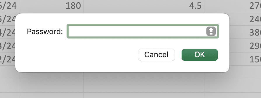
Step 1: Unprotect the worksheet.

• Go to the “Review” tab.
• Click “Unprotect Sheet“.

• Enter the password if prompted.

Step 2: Unlock specific cells.

• Select the cells you want to edit.
• Right-click and choose “Format Cells“.

• In the “Protection” tab, uncheck “Locked“.

• Click “OK” to apply.

Step 3: Make your changes.

• Edit the now-unlocked cells as needed.

Step 4: Re-protect the worksheet.

• Go back to “Review” > “Protect Sheet“.

• Set your protection options and password.

• Click “OK” to reapply protection.

Always remember to re-protect your worksheet after making changes to maintain the integrity of your data and formulas.

Mastering Cell Protection in Excel

Effective cell locking in Excel is crucial for maintaining data integrity and creating user-friendly spreadsheets. Experiment with different protection methods to find the best fit for your specific needs.

Ready to take your Excel skills to the next level? Coefficient offers powerful data integration features that complement Excel’s built-in protection capabilities. Get started with Coefficient to enhance your spreadsheet experience and streamline your data workflows.