Importing your Outreach Sequence records into Excel lets you measure cadence effectiveness, compare teams, and optimize outreach strategies. Follow this guide to install Coefficient, select the Sequence object, import your data, and automate refreshes.
TLDR
-
Step 1:
Step 1. In Excel, go to Insert → Get Add-ins → My Add-ins, search “Coefficient” and install.
-
Step 2:
Step 2. Launch Coefficient, choose “Import from Objects”, and pick “Sequence” under Outreach.
-
Step 3:
Step 3. Add filters on status or team, then click “Import”.
-
Step 4:
Step 4. (Optional) Schedule auto-refresh to keep sequence metrics live.


What Outreach Objects Are Available?
Account
- Opportunity
- Sequence
- Call Disposition
- Call Purpose
- Compliance Request
- Content Category
- Content Category Membership
- Content Category Ownership
- Duty
- Email Address
- Event
- Favorite
How to Import Workers Data from Rippling into Excel
Importing Workers data from Rippling into Excel helps HR teams track both employees and contractors, analyze workforce composition, and optimize labor costs. Coefficient makes this process simple and automatic.
This guide will show you how to import your Rippling Workers data into Excel using Coefficient.
TLDR
-
Step 1:
Step 1. Open Excel > Insert tab > Get Add-ins > Install Coefficient from Office Add-ins store.
-
Step 2:
Step 2. Connect your Rippling account and select the Workers object to import.
-
Step 3:
Step 3. (Optional) Enable auto-refresh to keep your data updated automatically.
Step 1: Install Coefficient in Excel and Connect Your Rippling Account
Begin by installing the Coefficient add-in in your Excel workbook:
- Open Excel and navigate to the Insert tab in the ribbon.
- Click on “Get Add-ins” to open the Office Add-ins store.
- Search for “Coefficient” and click “Add” to install it.
- Once installed, open the Coefficient sidebar by clicking on the Coefficient icon in the ribbon.
- Click on “Import from…” to see available data sources.
Step 2: Import Workers Data from Rippling
Now it’s time to connect to Rippling and import your Workers data:
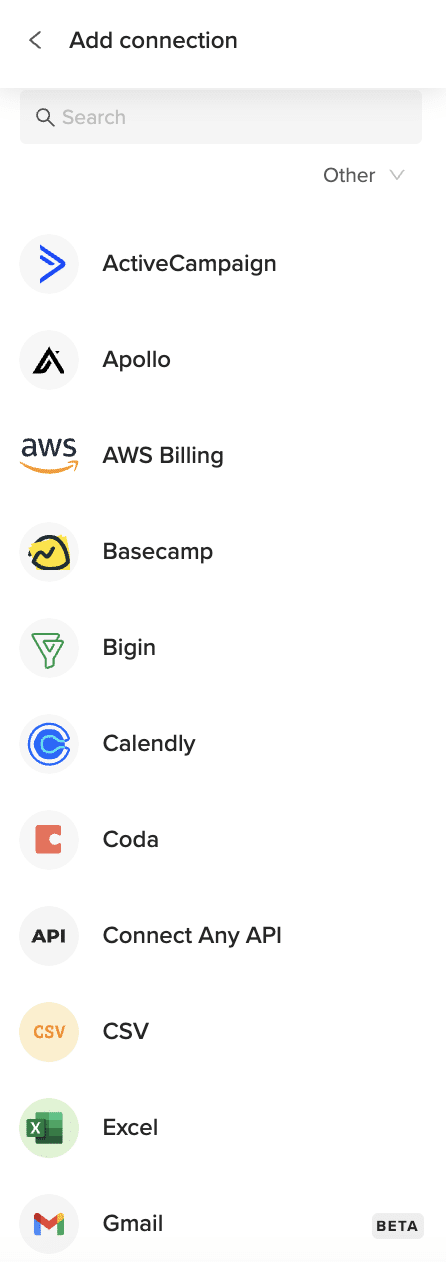
- In the Coefficient sidebar, navigate to the “Other” category.
- Find and select “Rippling” from the list of connectors.
- Log in to your Rippling account when prompted.
- Select “Workers” from the list of available objects.
- Configure any filters or select specific fields you want to import.
- Click “Import” to bring your Workers data into Excel.
Step 3: Set Up Auto-Refresh (Optional)
To ensure your Workers data stays up-to-date automatically:
- Hover over your imported data range in Excel.
- Click on the “Data Settings” icon that appears.
- Select “Schedule Refresh” from the menu.
- Choose your preferred refresh frequency (hourly, daily, or weekly).
- Set the specific timing for the refresh to occur.
- Click “Save” to confirm your auto-refresh settings.
Available Rippling Objects
- Workers
- Users
- Groups
- Departments
- Teams
- Levels
- Work Locations
- Company Activity
- Company Leave Types
- Leave Balances
- Leave Requests
How to Import Work Locations Data from Rippling into Excel
Importing Work Locations data from Rippling into Excel helps HR teams track office occupancy, analyze remote work patterns, and manage geographic workforce distribution. Coefficient makes this process simple and automatic.
This guide will show you how to import your Rippling Work Locations data into Excel using Coefficient.
TLDR
-
Step 1:
Step 1. Open Excel > Insert tab > Get Add-ins > Install Coefficient from Office Add-ins store.
-
Step 2:
Step 2. Connect your Rippling account and select the Work Locations object to import.
-
Step 3:
Step 3. (Optional) Enable auto-refresh to keep your data updated automatically.
Step 1: Install Coefficient in Excel and Connect Your Rippling Account
Begin by installing the Coefficient add-in in your Excel workbook:
- Open Excel and navigate to the Insert tab in the ribbon.
- Click on “Get Add-ins” to open the Office Add-ins store.
- Search for “Coefficient” and click “Add” to install it.
- Once installed, open the Coefficient sidebar by clicking on the Coefficient icon in the ribbon.
- Click on “Import from…” to see available data sources.
Step 2: Import Work Locations Data from Rippling
Now it’s time to connect to Rippling and import your Work Locations data:
- In the Coefficient sidebar, navigate to the “Other” category.
- Find and select “Rippling” from the list of connectors.
- Log in to your Rippling account when prompted.
- Select “Work Locations” from the list of available objects.
- Configure any filters or select specific fields you want to import.
- Click “Import” to bring your Work Locations data into Excel.
Step 3: Set Up Auto-Refresh (Optional)
To ensure your Work Locations data stays up-to-date automatically:
- Hover over your imported data range in Excel.
- Click on the “Data Settings” icon that appears.
- Select “Schedule Refresh” from the menu.
- Choose your preferred refresh frequency (hourly, daily, or weekly).
- Set the specific timing for the refresh to occur.
- Click “Save” to confirm your auto-refresh settings.
Available Rippling Objects
- Workers
- Users
- Groups
- Departments
- Teams
- Levels
- Work Locations
- Company Activity
- Company Leave Types
- Leave Balances
- Leave Requests
How to Import Teams Data from Rippling into Excel
Importing Teams data from Rippling into Excel helps managers track team compositions, analyze cross-functional collaboration, and optimize project staffing. Coefficient makes this process simple and automatic.
This guide will show you how to import your Rippling Teams data into Excel using Coefficient.
TLDR
-
Step 1:
Step 1. Open Excel > Insert tab > Get Add-ins > Install Coefficient from Office Add-ins store.
-
Step 2:
Step 2. Connect your Rippling account and select the Teams object to import.
-
Step 3:
Step 3. (Optional) Enable auto-refresh to keep your data updated automatically.
Step 1: Install Coefficient in Excel and Connect Your Rippling Account
Begin by installing the Coefficient add-in in your Excel workbook:
- Open Excel and navigate to the Insert tab in the ribbon.
- Click on “Get Add-ins” to open the Office Add-ins store.
- Search for “Coefficient” and click “Add” to install it.
- Once installed, open the Coefficient sidebar by clicking on the Coefficient icon in the ribbon.
- Click on “Import from…” to see available data sources.
Step 2: Import Teams Data from Rippling
Now it’s time to connect to Rippling and import your Teams data:
- In the Coefficient sidebar, navigate to the “Other” category.
- Find and select “Rippling” from the list of connectors.
- Log in to your Rippling account when prompted.
- Select “Teams” from the list of available objects.
- Configure any filters or select specific fields you want to import.
- Click “Import” to bring your Teams data into Excel.
Step 3: Set Up Auto-Refresh (Optional)
To ensure your Teams data stays up-to-date automatically:
- Hover over your imported data range in Excel.
- Click on the “Data Settings” icon that appears.
- Select “Schedule Refresh” from the menu.
- Choose your preferred refresh frequency (hourly, daily, or weekly).
- Set the specific timing for the refresh to occur.
- Click “Save” to confirm your auto-refresh settings.
Available Rippling Objects
- Workers
- Users
- Groups
- Departments
- Teams
- Levels
- Work Locations
- Company Activity
- Company Leave Types
- Leave Balances
- Leave Requests
How to Import Task Checklists Data from ClickUp into Excel
Getting your ClickUp Task Checklists data into Excel helps you analyze the breakdown and progress of tasks. Coefficient connects ClickUp directly to your spreadsheet.
This guide walks you through importing your ClickUp Task Checklists data into Excel using Coefficient.
TLDR
-
Step 1:
Step 1. Install Coefficient for Excel and connect your ClickUp account.
-
Step 2:
Step 2. Choose Import from… and select the Task Checklists object.
-
Step 3:
Step 3. Apply any necessary filters and import the data to your sheet.
-
Step 4:
Step 4. Set up an auto-refresh schedule to keep the data current.
Step-by-step guide
Follow these steps to bring your ClickUp Task Checklists data into Excel.
Step 1: Install and Connect Coefficient
To start, install the Coefficient add-in in Excel. Go to the Insert tab, click “Get Add-ins,” search for Coefficient, and install it from the store.
Open the Coefficient add-in from the Home tab. Select ClickUp when prompted to connect a data source.
Log in to your ClickUp account and authorize Coefficient to access your data.
Step 2: Import Task Checklists Data
With ClickUp connected, click “Import from…” in the Coefficient sidebar.
Select ClickUp, then choose “Task Checklists” from the list of objects to import.
You can select specific checklist fields or filter the data as needed before clicking “Import” to bring it into your Excel sheet.
Step 3: Set Up Auto-Refresh (Optional)
Keep your Task Checklists data in Excel automatically updated by setting up auto-refresh. Find the auto-refresh settings in the Coefficient sidebar after importing.
Schedule refreshes hourly, daily, or weekly. Your Excel sheet will then automatically sync with the latest task checklist information from ClickUp.
Available ClickUp Objects
- Authorization
- Attachments
- Comments
- Custom Task Types
- Custom Fields
- Docs
- Folders
- Goals
- Guests
- Lists
- Members
- Roles
How to Import Task Relationships Data from ClickUp into Excel
Importing your ClickUp Task Relationships data into Excel helps you analyze dependencies and links between tasks. Coefficient provides a direct connection to your spreadsheet.
This guide shows you how to import your ClickUp Task Relationships data into Excel using Coefficient.
TLDR
-
Step 1:
Step 1. Install Coefficient for Excel and link your ClickUp account.
-
Step 2:
Step 2. Click Import from… and choose the Task Relationships object.
-
Step 3:
Step 3. Configure filters or select specific fields and import the data.
-
Step 4:
Step 4. Enable auto-refresh for automatic data updates on a schedule.
Step-by-step guide
Here is how to get your ClickUp Task Relationships data into Excel.
Step 1: Install and Connect Coefficient
First, install the Coefficient add-in. In Excel, go to the Insert tab, click “Get Add-ins,” search for Coefficient, and install it from the store.
Open the Coefficient add-in from the Home tab. When asked to connect a data source, select ClickUp.
Log in to your ClickUp account and grant Coefficient access to your data.
Step 2: Import Task Relationships Data
With ClickUp connected, click “Import from…” in the Coefficient sidebar.
Select ClickUp as your source. Then, choose “Task Relationships” from the list of available objects to import.
You can refine the data by selecting specific fields or applying filters before clicking “Import” to add it to your Excel sheet.
Step 3: Set Up Auto-Refresh (Optional)
Keep your Task Relationships data in Excel automatically updated. After importing, find the auto-refresh options in the Coefficient sidebar.
Schedule refreshes hourly, daily, or weekly. Your Excel sheet will then sync automatically with the latest task relationship information from ClickUp.
Available ClickUp Objects
- Authorization
- Attachments
- Comments
- Custom Task Types
- Custom Fields
- Docs
- Folders
- Goals
- Guests
- Lists
- Members
- Roles
How to Import Tables Data from BigQuery into Excel
Accessing your BigQuery Tables data in Excel allows for straightforward data analysis without complex tools. Coefficient connects BigQuery directly to your spreadsheet.
This guide shows you how to import your BigQuery Tables data into Excel using Coefficient.
TLDR
-
Step 1:
Step 1. Install Coefficient for Excel and connect to your BigQuery account.
-
Step 2:
Step 2. Select Import from… and choose the Tables object.
-
Step 3:
Step 3. Configure filters or select fields as needed and import into your Excel sheet.
-
Step 4:
Step 4. Set up auto-refresh to keep your table data automatically updated.
Step-by-step guide
Follow these steps to bring your BigQuery Tables data into Excel.
Step 1: Install and Connect Coefficient
First, install Coefficient for Excel. Go to the Insert tab, click “Get Add-ins,” search for Coefficient, and install it from the store.
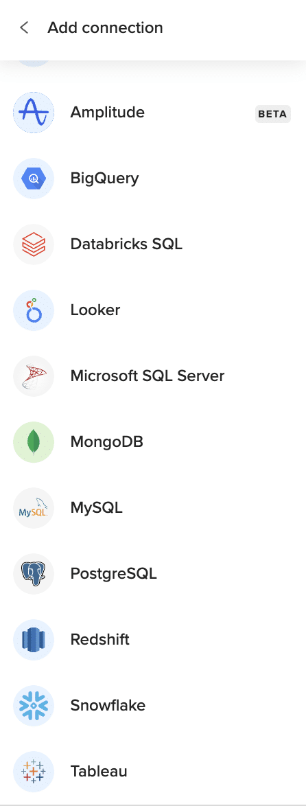
Open the Coefficient add-in from the Home tab. Select BigQuery when prompted to connect a data source.
Log in to your BigQuery account and authorize Coefficient to access your data.
Step 2: Import Tables Data
With BigQuery connected, click “Import from…” in the Coefficient sidebar.
Select BigQuery as your source. Then, choose “Tables” from the list of available objects to import.
You can refine the data by selecting specific fields or applying filters before clicking “Import” to add it to your Excel sheet.
Step 3: Set Up Auto-Refresh (Optional)
Keep your Tables data in Excel automatically updated. After importing, find the auto-refresh options in the Coefficient sidebar.
Schedule refreshes hourly, daily, or weekly. Your Excel sheet will then sync automatically with the latest table information from BigQuery.
Available BigQuery Objects
- Columns
- SQL
How to Import SQL Data from BigQuery into Excel
Importing data from BigQuery using SQL queries into Excel gives you flexibility for custom reports. Coefficient makes running SQL and getting results into your spreadsheet easy.
This guide shows you how to import your BigQuery SQL data into Excel using Coefficient.
TLDR
-
Step 1:
Step 1. Install Coefficient for Excel and connect to your BigQuery account.
-
Step 2:
Step 2. Select Import from… and choose the SQL option.
-
Step 3:
Step 3. Write or paste your SQL query and import the results into your Excel sheet.
-
Step 4:
Step 4. Set up auto-refresh to keep your query results automatically updated.
Step-by-step guide
Here is how to get your BigQuery SQL data into Excel.
Step 1: Install and Connect Coefficient
First, install the Coefficient add-in. In Excel, go to the Insert tab, click “Get Add-ins,” search for Coefficient, and install it from the store.
Open the Coefficient add-in from the Home tab. When asked to connect a data source, select BigQuery.
Log in to your BigQuery account and grant Coefficient access to your data.
Step 2: Import SQL Data
With BigQuery connected, click “Import from…” in the Coefficient sidebar.
Select BigQuery as your source. Then, choose “SQL” from the list of available import options.
Write or paste your SQL query into the Coefficient interface. Configure any options needed, then click “Import” to add the query results to your Excel sheet.
Step 3: Set Up Auto-Refresh (Optional)
Keep your SQL query results in Excel automatically updated. After importing, find the auto-refresh options in the Coefficient sidebar.
Schedule refreshes hourly, daily, or weekly. Your Excel sheet will then sync automatically by re-running your SQL query in BigQuery.
Available BigQuery Objects
- Columns
- SQL
How to Import Members Data from ClickUp into Excel
Getting your ClickUp Members data into Excel helps you manage and track team member information effectively. Coefficient connects ClickUp directly to your spreadsheet.
This guide walks you through importing your ClickUp Members data into Excel using Coefficient.
TLDR
-
Step 1:
Step 1. Install Coefficient for Excel and connect your ClickUp account.
-
Step 2:
Step 2. Choose Import from… and select the Members object.
-
Step 3:
Step 3. Apply any necessary filters and import the data to your sheet.
-
Step 4:
Step 4. Set up an auto-refresh schedule to keep the data current.
Step-by-step guide
Follow these steps to bring your ClickUp Members data into Excel.
Step 1: Install and Connect Coefficient
To start, install the Coefficient add-in in Excel. Go to the Insert tab, click “Get Add-ins,” search for Coefficient, and install it from the store.
Open the Coefficient add-in from the Home tab. Select ClickUp when prompted to connect a data source.
Log in to your ClickUp account and authorize Coefficient to access your data.
Step 2: Import Members Data
With ClickUp connected, click “Import from…” in the Coefficient sidebar.
Select ClickUp, then choose “Members” from the list of objects to import.
You can select specific member fields or filter the data as needed before clicking “Import” to bring it into your Excel sheet.
Step 3: Set Up Auto-Refresh (Optional)
Keep your Members data in Excel automatically updated by setting up auto-refresh. Find the auto-refresh settings in the Coefficient sidebar after importing.
Schedule refreshes hourly, daily, or weekly. Your Excel sheet will then automatically sync with the latest member information from ClickUp.
Available ClickUp Objects
- Authorization
- Attachments
- Comments
- Custom Task Types
- Custom Fields
- Docs
- Folders
- Goals
- Guests
- Lists
- Members
- Roles
How to Import Leave Requests Data from Rippling into Excel
Importing Leave Requests data from Rippling into Excel helps HR teams track time-off patterns, analyze absence trends, and plan for workforce coverage. Coefficient makes this process simple and automatic.
This guide will show you how to import your Rippling Leave Requests data into Excel using Coefficient.
TLDR
-
Step 1:
Step 1. Open Excel > Insert tab > Get Add-ins > Install Coefficient from Office Add-ins store.
-
Step 2:
Step 2. Connect your Rippling account and select the Leave Requests object to import.
-
Step 3:
Step 3. (Optional) Enable auto-refresh to keep your data updated automatically.
Step 1: Install Coefficient in Excel and Connect Your Rippling Account
Begin by installing the Coefficient add-in in your Excel workbook:
- Open Excel and navigate to the Insert tab in the ribbon.
- Click on “Get Add-ins” to open the Office Add-ins store.
- Search for “Coefficient” and click “Add” to install it.
- Once installed, open the Coefficient sidebar by clicking on the Coefficient icon in the ribbon.
- Click on “Import from…” to see available data sources.
Step 2: Import Leave Requests Data from Rippling
Now it’s time to connect to Rippling and import your Leave Requests data:
- In the Coefficient sidebar, navigate to the “Other” category.
- Find and select “Rippling” from the list of connectors.
- Log in to your Rippling account when prompted.
- Select “Leave Requests” from the list of available objects.
- Configure any filters or select specific fields you want to import.
- Click “Import” to bring your Leave Requests data into Excel.
Step 3: Set Up Auto-Refresh (Optional)
To ensure your Leave Requests data stays up-to-date automatically:
- Hover over your imported data range in Excel.
- Click on the “Data Settings” icon that appears.
- Select “Schedule Refresh” from the menu.
- Choose your preferred refresh frequency (hourly, daily, or weekly).
- Set the specific timing for the refresh to occur.
- Click “Save” to confirm your auto-refresh settings.
Available Rippling Objects
- Workers
- Users
- Groups
- Departments
- Teams
- Levels
- Work Locations
- Company Activity
- Company Leave Types
- Leave Balances
- Leave Requests