Understanding The Excel INDEX Function: Real World Examples

Introduction To The Excel INDEX Function

The Excel Index Function is a significant tool that can modify the way you manage data. Whether you’re a beginner or recurring Excel user, grasping this function can substantially boost your effectiveness and precision in handling spreadsheets. The INDEX Function permits you to extract concrete data from large sets of data based on your norms, making it necessary for anyone handling comprehensive lists or tables.

In this article, we will discuss the variations of the INDEX function, discover its practical examples, and show you how it can simplify intricate data tasks.

Let’s dive in.

Array And Reference Forms Of The Excel INDEX Function

Both forms of the INDEX function may look similar, but they vary in their syntax, arguments, and use.

INDEX Function Syntax
Array Form	Reference Form
=INDEX(array, row_num, [column_num])	=INDEX(reference, row_num, [column_num], [area_num] )

Next, let’s look at how to correctly use the arguments in both the forms.

INDEX Function Arguments
	Array Form	Reference Form
array/reference	array is a single range of cells from which you want to retrieve data.	reference could be a single or multiple ranges of cells from which you want to retrieve data.
row_num	It is the row number in the array/reference from which to return a value.
[column_num]	It is an optional field where you can enter the column number from which to return a value.
[area_num]	–	It is an optional field where you can specify which reference range you want to run the INDEX function in.

One thing to note is that if you want to find a specific cell in a column (instead of a row), you may set the row_num value to “0,” and instead specify the column_num value.

Don’t worry if this seems a little confusing. Some examples will help clarify how to use the INDEX Function in Excel.

Note: The syntax, arguments, and following examples are for using the INDEX function in Excel. If you’d like to learn about using the INDEX function in Google Sheets, check out our ultimate guide on using INDEX in Google Sheets.

Video Tutorial

Check out the tutorial below for a complete video walkthrough!

Practical Examples Of The Excel INDEX Function

Example #1: Array Form

Let’s say you’re a mobile phone manufacturer who makes three kinds of phones (Basic Phone, Smartphone, Foldable Smartphone) and you have the quarterly sales data for each product for the last financial year.

If you want to retrieve the sales figure for “Smartphone” for Q3, you can use the INDEX Function by specifying the following arguments:

• array: D4:D6, since this array contains all Q3 sales figures. 
• row_num: 2, since “Smartphone” is the second row.
• column_num: Not needed, since the array we’ve specified is a single column.

So the INDEX function in this case will be: =INDEX(D4:D6, 2)

This will return the value in cell D5.

Next, let’s see how to use the reference form of the INDEX function.

Example #2: Reference Form

Let’s assume you’re the mobile phone manufacturer from the previous example, but you’re looking at sales figures across two countries.

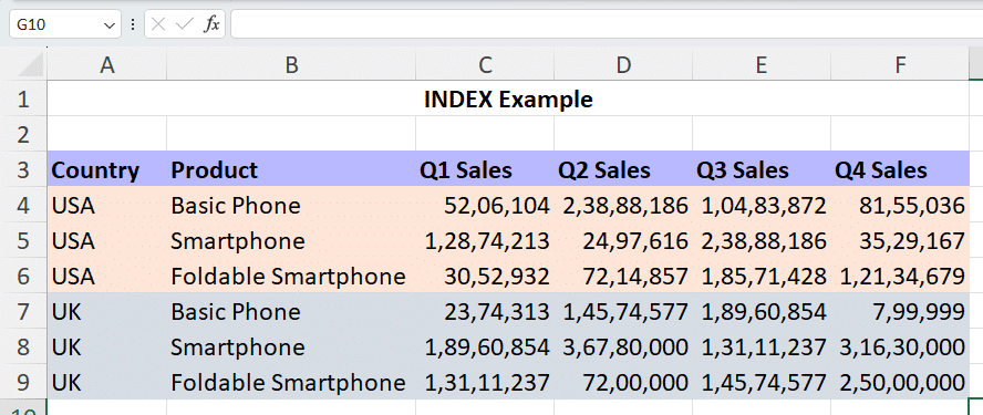
In this example, there are 2 distinct arrays, one for each country. So, to retrieve the “Basic Phone” sales in UK, for Q2, you can use the INDEX function with the following arguments:

• reference: (A4:F6,A7:F9), since these are the 2 sets of arrays.
• row_num: 1, since “Basic Phone” is the first row in each array.
• column_num: 4, since this column contains the Q2 sales figures.
• area_num: 2, since UK sales figures are in the second array.

So the INDEX function in this case will be: =INDEX((A4:F6,A7:F9),1,4,2)

This will return the value in cell D7.

We hope that clears up any doubt you might have had regarding how to use the INDEX function in both array and reference forms.

However, it is not uncommon to run into errors when dealing with larger datasets. The most common among these is the #REF! error.

Addressing The #REF! Error When Using The Excel INDEX Function

Sometimes you’ll run into the #REF! error when using the INDEX function in Excel.

Don’t worry! This just means you’ve entered a wrong value in one of the arguments.

When you enter a value outside the range of the specified array or reference, you’ll run into the #REF! error.

In this example, we entered 4 as the row_num argument. But the specified references only have 3 rows each.

Hence, we run into the #REF! error.

Correct this mistake by entering a valid row number and you’ll be able to kick this error to the curb.

So now you know how to use the INDEX function and troubleshoot the most common error. But wait, we’re just getting started!

In the next section, we’ll explore how you can gain advanced functionality by using the INDEX function with other functions.

Combining The Excel INDEX Function With Other Functions

Let’s look at how the INDEX function can supercharge some common functions.

1. Using INDEX With SUM/AVERAGE

You can use the INDEX function within the SUM or AVERAGE functions to either get the sum or average of select values within a row/column. Or even to calculate the sum or average of 2 specific cells.

Let’s look at an example of this.

Example: Calculating SUM/AVERAGE of Select Values using INDEX

Let’s say your data set looks like this:

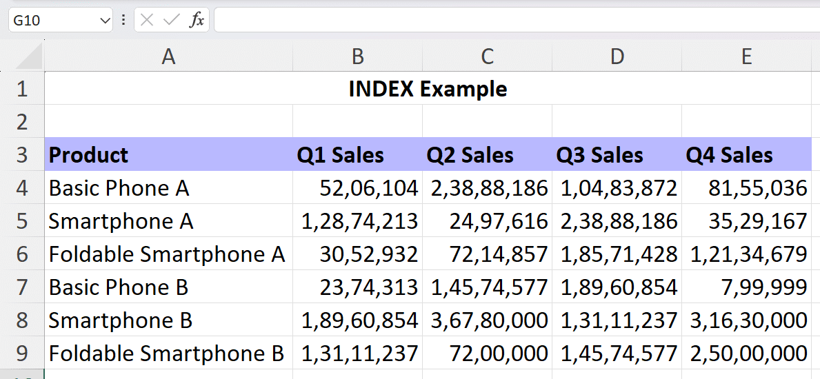
And you want to calculate the total sales of Smartphone B + Foldable Smartphone B in Q2 and Smartphone A + Foldable Smartphone A in Q3. Instead of specifically selecting those cells to calculate the sum, you can use the INDEX function like this:

=SUM(INDEX(C8:C9,0,1),INDEX(D5:D6,0,1))

You’ll notice that the row_num argument is set to 0 and the column_num argument is set to 1 in both the INDEX functions within SUM. This is because instead of specifying certain cells within both arrays, we want to sum the entire array.

You may be wondering why not use the SUM function by specifying the cells directly.

The advantage of using the INDEX function in such a case is that if you want to calculate the sum of a different set of cells, you don’t need to write a new function.

You can modify the existing function or just copy it into a new cell, and change the arguments within the INDEX functions. Like so:

You’ll notice we’ve changed the summation function to: =SUM(INDEX(B7:B9,0,1),INDEX(E4:E6,0,1))

This will calculate the sum of all “B” products in Q1 and all “A” products in Q4, without having to write a completely new SUM function specifying those cells.

You can substitute SUM with AVERAGE, and use the INDEX function in a similar fashion.

2. Using INDEX With MIN/MAX

You can use the INDEX function with MIN/MAX to get additional functionality, without having to rewrite functions over and over. Let’s see an example of that.

Example: Calculating MIN/MAX of Specific Ranges using INDEX

We’ll use the same data set as in the previous section and use the function: =MAX(INDEX(B4:B9,0),INDEX(E4:E9,0))

This will output the maximum value of the two ranges specified in the INDEX functions within the MAX function.

You could simply swap the MAX to MIN or change the cell ranges within which you want to calculate MIN/MAX, just by changing the arguments in the function.

These are just a few of the ways the INDEX function can make simple calculations more powerful and versatile.

In the next section, we’ll take a peek into how using the INDEX-MATCH function can simplify even advanced data analysis operations.

3. Enhancing Functionality With Excel INDEX & MATCH

The INDEX-MATCH functionality can significantly cut down the time required for complex data analytics tasks. Let’s explore this with an example.

Example: Using INDEX-MATCH to Retrieve Relevant Data

Following on from the example in the previous section, let’s say we’ve identified the highest sales of a single product in Q1 by using the INDEX function with the MAX function.

But now, we want to find out which product this sales figure belongs to.

We’ll use the INDEX-MATCH function to do so. Let’s break down the exact function and parameters we need to achieve this:

• We want the function to return a product name, which is located somewhere in the range A4:A9. Hence, that becomes the array argument.
• The next argument is row_num, which we’ll identify using the MATCH function.
• The first argument for the MATCH function is lookup_value, which we’ve already identified in cell G4 (i.e., highest sales of a single product in Q1 ).
• The second argument for the MATCH function is lookup_array, which is the range in which the lookup_value is located. In this case, all the Q1 sales figures, B4:B9.
• Finally, we want an exact match for the lookup_value, so we’ll use 0 for the match_type.

So the final function will be: =INDEX(A4:A9,MATCH(G4,B4:B9,0))

Hit enter and you should see the product name corresponding to the sales figure in cell G4.

4. Extracting Meaningful Data using Drop-Down Lists and INDEX

If you thought the previous example was powerful, wait till you see this one. We’ll use the INDEX-MATCH function and combine it with Excel’s drop-down lists to extract exactly the data we want.

Let’s explore this with a simple example.

Example: Using INDEX Function with Drop-Down Lists

Let’s use the data set from the very first example in this article.

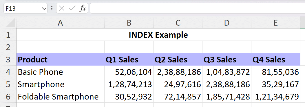
Now, if you had to calculate the annual sales of each product, you could do a simple SUM function for each product and add it in Column F.

Or you could create a drop-down list for all the Products.

Now, we could use the INDEX function within the SUM function to calculate the annual sales of each product, but that would still require copying/modifying the function three times (once for each product).

But a better way would be to define an INDEX function that returns the total of each row, based on which product you select in cell G4 (where the drop-down is located).

Thus, the function would be: =SUM(INDEX((B4:E4,B5:E5,B6:E6),0,0,MATCH(G4,A4:A6,0)))

Note:

• We’ve used the INDEX function within the SUM function to calculate the total of each quarter’s sales.
• We’ve used the Reference form of the INDEX function to define three distinct arrays for each product.
• We’ve set the row_num argument as 0, since there is only one row in each array.
• We’ve set the column_num argument as 0, since we want the INDEX function to return all the values in the array.
• Instead of defining the area_num argument directly, we’ve used the MATCH function to return a value based on the drop-down selected in cell G4.

Now, all you need to do is select the product from the drop-down list to see its annual sales in cell H4. How nifty is that!

5. Creating a Dynamic Chart Data Range

One of the advanced applications of the Excel INDEX Function is energetic range selection, which permits you to create dynamic formulas that adjust based on your data. This can be specifically useful when handling variable data spectrums, where the amount of data might alter constantly.

Step By Step Guide:

Step 1: Prepare your Data

Ensure that your data is arranged with the months in one column (e.g, Column A) and the sales figures in another column (e.g., Column B).

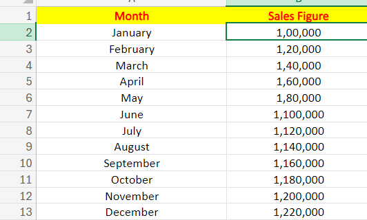
Depicted Name Ranges: Create name ranges utilizing the INDEX function to dynamically adapt the data range.

• Go to the ‘Formulas’ tab and choose ‘Name Manager’.
• Click ‘New’ to create a new named range.
• Name the r

  

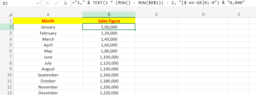
Applying this formula helps to create a dynamic range that indulges all non-empty cells in the Column A.

Step 2: Create the Chart

• Choose the range of data for the chart using the named ranges. Go to ‘Insert’ and select the type of chart you want (e.g., Line Chart)
• In the data range of Chart, enter:

‘Sheet1’!A1:B13

This will inform Excel to use the Dynamic ranges for the data of the chart.

Step 3: Test the Dynamic Range

• Add new data to the set of data to examine if the chart updates involuntarily. The chart should adapt to indulge the new months and figures of sales without any extra manual updates.

Using The Excel INDEX Function

The INDEX function in Excel may seem limited in scope at a glance, but it offers a powerful and efficient way to retrieve data from large data sets.

Grasping the INDEX Excel function opens up a globe of potentials for effective data handling. Its capability to identify and recover precise data from wide datasets makes it indispensable for both everyday tasks and intricate data analysis. By incorporating the INDEX Function into your Excel toolkit, you can smoothen your workflow, improve your productivity, and confront data difficulties with confidence.

Now that you comprehend how to use this significant function, you’re well on your way to becoming a Pro in Excel. Keep working on Excel, and observe as your data managing expertise reaches new heights.

If you’d like to avoid hours of repetitive tasks and become even more efficient in Excel, check out Coefficient’s sidebar app and automation tool for Excel. Sync data from your CRM, database, ad platforms, and more into Excel with just a few clicks. Get started today!