How to Highlight or Remove Duplicates in Google Sheets

The following is a comprehensive guide on how to highlight and remove duplicates in Google Sheets.

Duplicate data compromises the quality and accuracy of your performance metrics, sales dashboards, decision-making, and other mission-critical efforts. That’s why you need an efficient data cleanup method to highlight and remove duplicates in Google Sheets.

Also, watch our video tutorial below for a complete guide on how to highlight duplicates in Google Sheets.

Video Tutorial: How to Highlight Duplicates in Google Sheets

Prerequisites for Highlighting Duplicates in Google Sheets

Before attempting to highlight duplicates in Google Sheets, try to ensure the following:

• Eliminate other conditional formatting rules currently applied to the cell you’re targeting
• Make sure you don’t have missing spaces in your searches
• Do not select headers when highlighting duplicates with Array Formulas
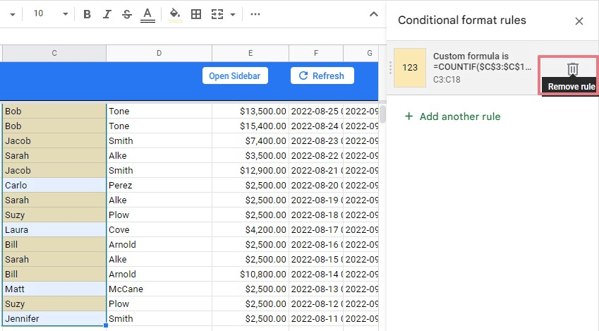
• Avoid highlighting specified duplicate values if necessary. Select the cells with the conditional formatting rule. Then click the trash icon under Format > Conditional formatting.

Here’s another pitfall to watch out for. Google Sheets can fail to highlight duplicates due to extra space characters.

This is when there are extra spaces — trailing or leading spaces — around the text in one cell but not in another. This can result in missed duplicates, since Google Sheets searches for an exact match.

You can remove extra spaces in your cells by using the TRIM or CLEAN functions in Google Sheets.

5 Ways to Highlight Duplicates in Google Sheets

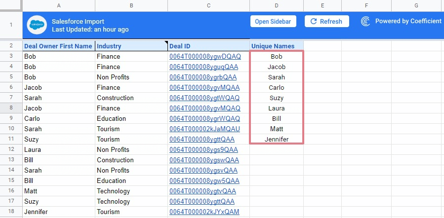
In Google Sheets, you can use custom formulas paired with conditional formatting to highlight duplicates. We’ll use a Salesforce dataset to perform the step-by-step walkthroughs below.

1. Highlight duplicates in a single column

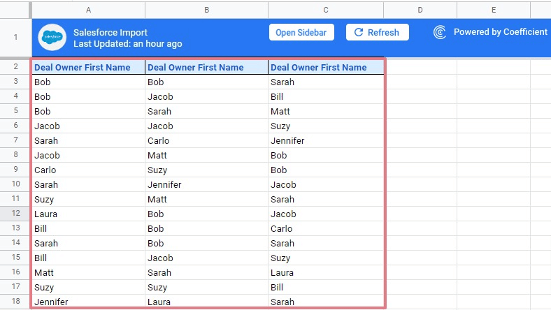
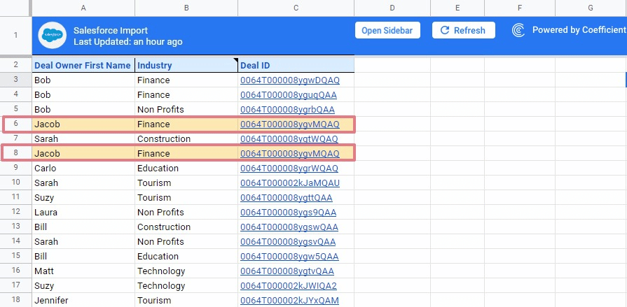
Highlighting duplicates in a single column is very straightforward. Suppose you want to highlight the duplicate entries in the Deal Owner First Name column.

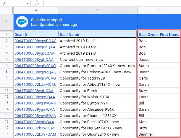
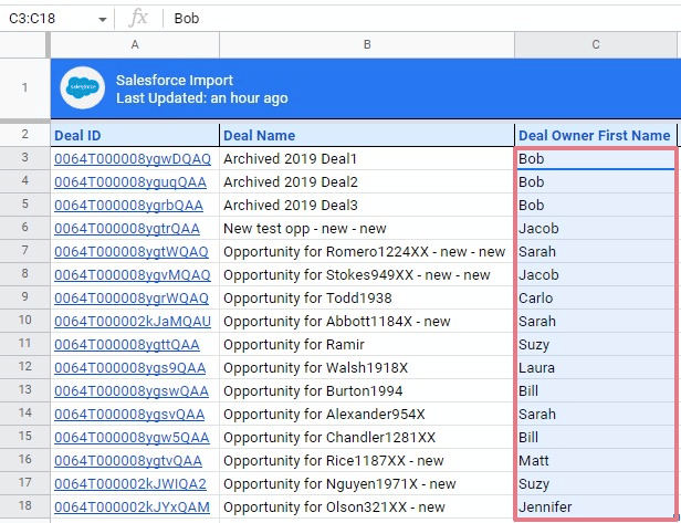
Step 1: First, select the column in the dataset (excluding the headers).

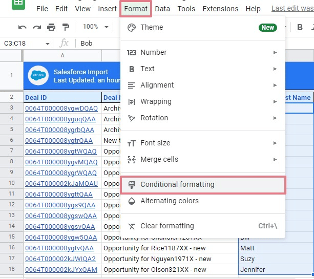
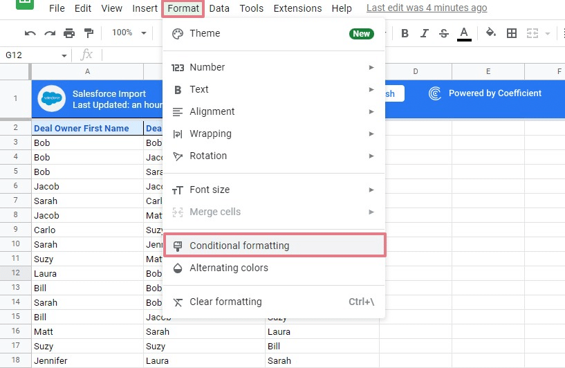
Step 2: Click Format in the top menu and select Conditional Formatting from the dropdown.

Step 3: Click Add another rule on the Conditional format rules side panel.

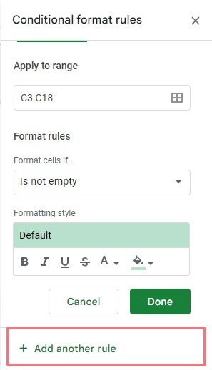
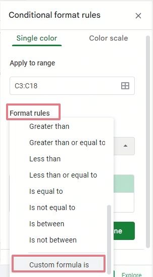
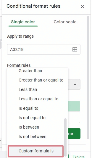
Step 4: Under Format rules, click Format cells if… and select Custom formula is from the drop down menu. Now, let’s write our first Google Sheet duplicate formula.

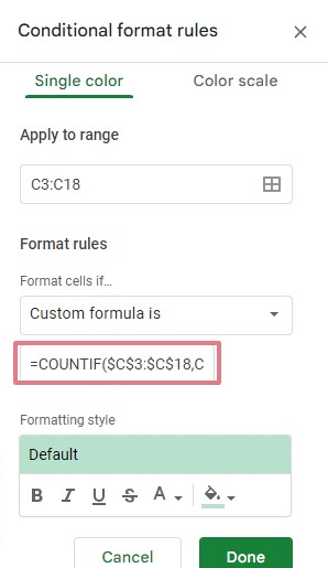
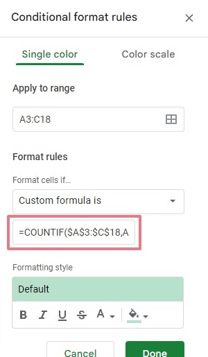
Step 5: Enter the COUNTIF formula under the Format cells if… field.
=COUNTIF($C$3:$C$18,C3)>1

Check out our Ultimate Guide to COUNTIF in Google Sheets blog if you want to learn more about this function.

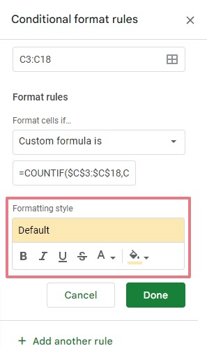
Step 6: Set the formatting style to highlight duplicates and click Done.

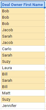
You will see the duplicate names highlighted in the column range in your set color and format.

Conditional formatting is also dynamic. It means you can change the data in any cell within your range, and the formatting will update automatically.

For instance, if you remove one of the two Suzys from the column range, Google Sheets will automatically stop highlighting Suzy since the name is no longer duplicated.

You can remove the highlight on a duplicate value by selecting the cell (or cells) and deleting the conditional formatting rule.

2. Highlight duplicates in multiple columns

You can also use conditional formatting to find duplicates in multiple columns of Google Sheets.

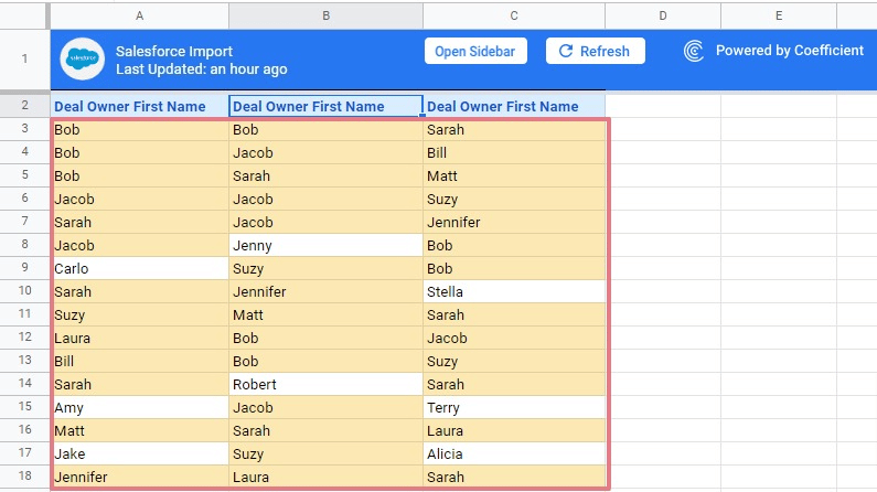
For example, let’s say you have three columns, all containing duplicate data.

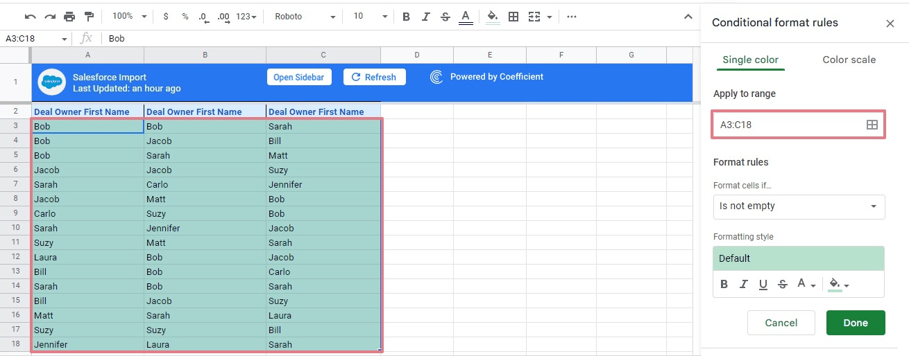
Follow the same steps from the previous example. Select the data range (excluding headers) and click Format > Conditional formatting.

Select Add another rule on the Conditional format rules side panel.

Double check the range of cells. Make sure it includes all the columns you want to find duplicates in.

Click the Format cells if… option and select Custom formula is.

Enter the following formula in the designated field.

=COUNTIF($A$3:$C$18,A3)>1

Set your preference in the formatting style section for highlighting duplicate data and click Done. The duplicate names that appear across these three columns are now highlighted.

3. Highlight duplicate rows

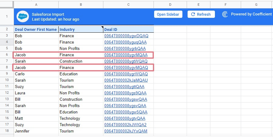
It’s a bit trickier to highlight duplicate rows. For instance, in the Salesforce dataset below, rows six and eight are duplicated. All the corresponding cells contain the same data.

To find duplicate rows, you should execute the steps from the previous example, but with modifications to the Custom formula is:

• Step 1: Select your data range, but not the header row
• Step 2: Open the Conditional formatting option and the Conditional format rules side panel from the Format top menu
• Step 3: Click Add another rule
• Step 4: Select Custom formula is from the Format cells if… dropdown list
• Input the following formula in the Value or formula field: =COUNTIF(ARRAYFORMULA($A$3:$A$18&$B$3:$B$18&$C$3:$C$18),$A3&$B3&$C3)>1
• Step 5: Choose your preferred formatting style and color for your highlighted duplicates and Click Done

You should see rows six and eight highlighted, since these contain repeating cell values.

A quick explanation of this method:

The conditional formatting formula in this example works the same as in the others. The formula highlights duplicate cells within a column. However, the formula combines all the rows’ content and makes a single string for each row.

This part of the formula: ARRAYFORMULA($A$3:$A$18&$B$3:$B$18&$C$3:$C$18)  creates an array of strings where the cells’ content within a row are combined. Concatenation is performed using the ampersand.

The COUNTIF formula uses the array. The condition is a concatenated string with all the values in a row, appearing like this:

$A3&$B3&$C3

The array is essentially a column-type construct. The COUNTIF function checks the number of times the combined string repeats in the array.

The end result: the formula highlights all the duplicate rows from the unique rows in the specified cell range.

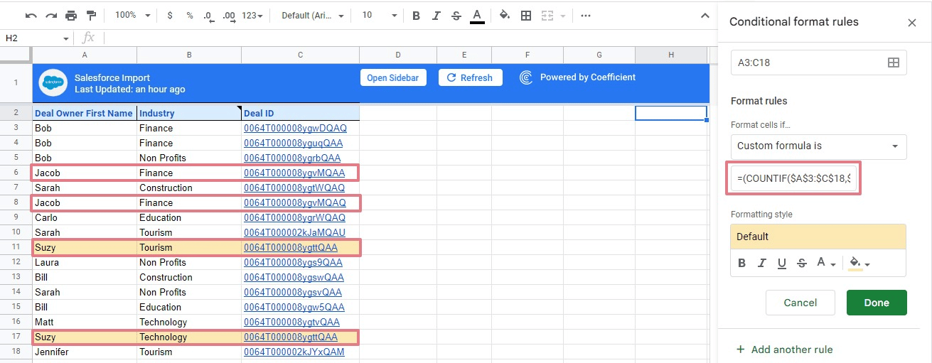
4. Highlight duplicates using added criteria

You can use added criteria in Google Sheets to highlight duplicate data. For example, you can configure your Sheet to only highlight duplicates for specific values.

Your syntax should include the star operator (“*”) to tell the COUNTIF function to use both criteria. The complete syntax will look like this:

=(COUNTIF(Range,Criteria)>1) * (New Condition) )

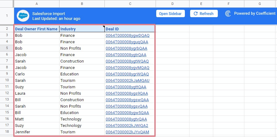
Let’s look again at the dataset from the previous example. There are two employees named Jacob with different Deal IDs.

In this case, we will highlight the duplicate employees, and also add a second condition for the Deal ID.

First, follow the same steps as our previous examples. When you get to the Conditional format rules side panel, input this formula:

=(COUNTIF($A$3:$C$18,$A3)>1)

Then you’ll need to this formula to account for the Deal ID:

1. • Place the “*” operator after the initial formula
   • Add the second condition to your (COUNTIF(Range,Criteria)>1) syntax
   • Your whole complete formula should look like this: =(COUNTIF($A$3:$C$18,$A3)>1)*(COUNTIF($A$3:$C$18,$C3)>1)

Of course, you can keep fine tuning your formula for the conditional format rules:

1. • Add a third criteria
   • Place another argument after the criteria (e.g., <5 or >0)
   • Insert several other “*” conditions

5. Highlight duplicates using the UNIQUE function

A UNIQUE formula finds all the unique values within a cell range. The function works best with a smaller dataset.

The syntax is simple: =UNIQUE(Range)

Let’s apply this function to the same dataset, so we can find unique values.

Select an empty cell. Type in =UNIQUE and include the data range you want to check for unique data:

=UNIQUE(A3:A18)

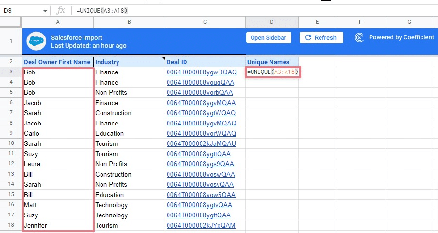
The formula will return the unique values within A3:A18.

UNIQUE eliminates complicated formula configurations and provides you with a clean dataset without duplicates. However, in more advanced duplicate use cases, this function alone can run into limitations.

How to Remove Duplicates in Google Sheets?

If you just want to remove duplicates from a range, Google Sheets has made it super easy with a built-in function requiring no complex formulas or conditions to add. Follow the quick step-by-step walkthrough here,

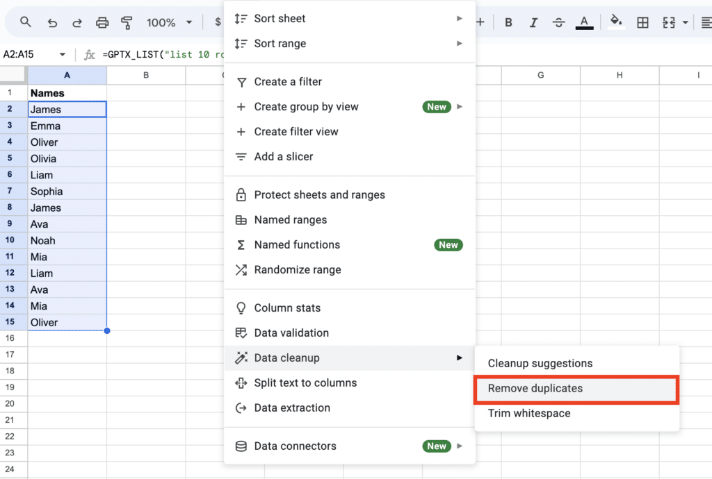
Step 1: Select the range from which you want to delete duplicates.

Step 2: Click Data in the toolbar above. Navigate to Data Cleanup and select “Remove Duplicates”.

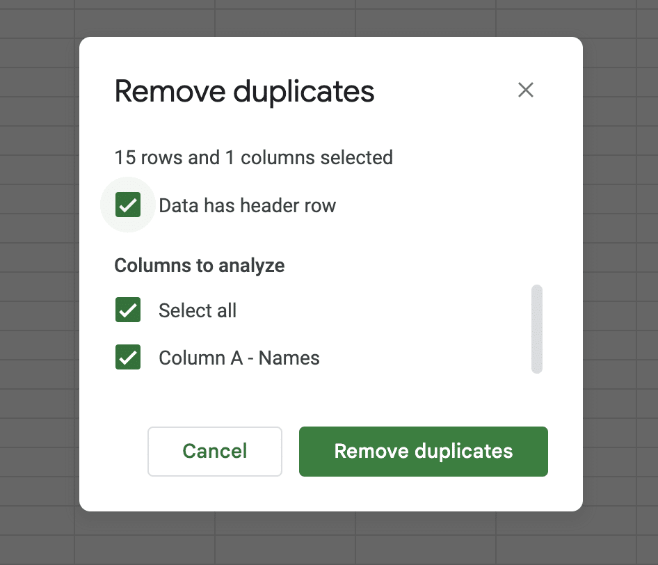
Step 3: Confirm your range settings and adjust if you have a header row or not.

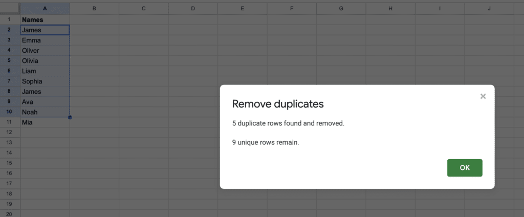
Step 4: Google Sheets completes removing duplicates and shows a summary like number of duplicates removed.

Use AI to Write Formulas for Conditional Formatting

As you can see, there are quite a few alternatives to highlight duplicates within Google Sheets. But you don’t have to go at it alone.

You can use Coefficient’s free GPT Copilot to automatically generate any spreadsheet formula, pivot, or chart, including your conditional formatting formulas. To use GPT Copilot, you need to install Coefficient. The install process takes less than a minute.

Once the installation is finished, return to Extensions on the Google Sheets menu. Coefficient will be available as an add-on.

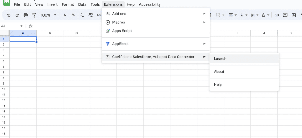
Step 1: Now launch Coefficient app from Google Sheets Add-on. Coefficient will run on the sidebar. Select GPT Copilot on the sidebar.

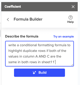
Step 2: Then click Formula Builder.

Step 3: Type a description of a formula into the text box. To recreate one of our conditional formatting formulas above, let’s highlight deals if the deal owner’s name and deal ID are both the same on multiple rows. Let’s type: Write a conditional formatting formula to highlight duplicate rows if both of the values in column A AND C are the same in both rows in sheet11.

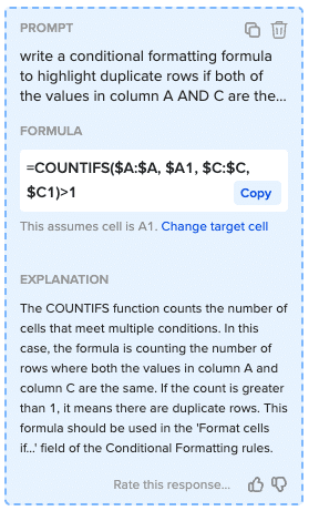
Step 4: Then press ‘Build’. Formula Builder will automatically generate the formula from the first example.

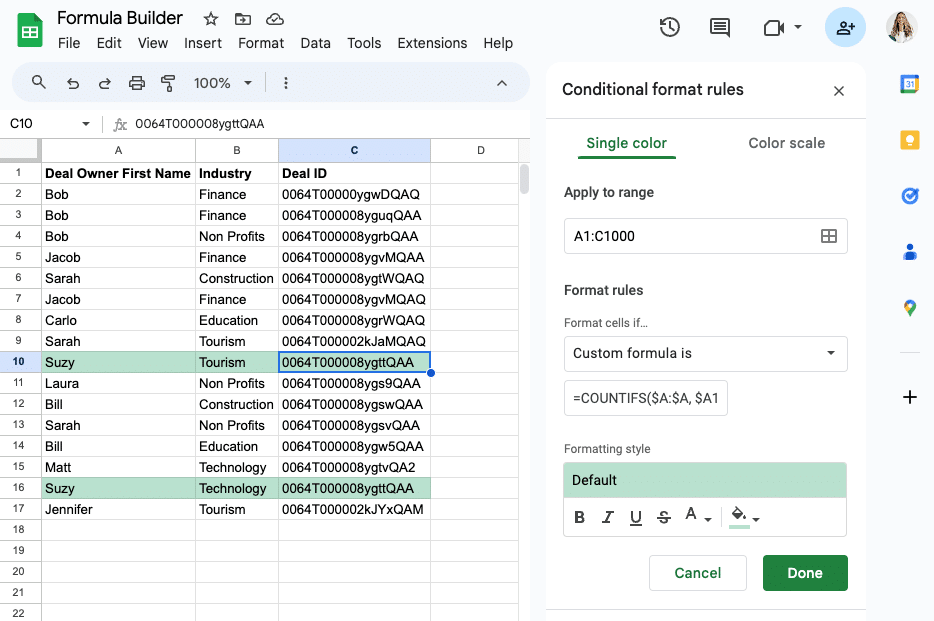
Step 5: Simply open up Conditional Formatting in the Format dropdown, add a new rule, select Custom Formula and paste your conditional formatting formula.

Highlight Duplicates in Google Sheets to Improve Data Quality

Your spreadsheet data impacts your metrics, reporting, analysis, and decision-making at every level. With Google Sheets, it’s easy to highlight and remove duplicates, improving data quality for your business operations. The methods outlined in this blog are simple yet effective ways to ensure superior data.