How to Create Dynamic Hyperlinks in Google Sheets

This guide will walk you through the process of creating and managing dynamic hyperlinks in Google Sheets, from basic techniques to advanced methods.

Basic Method: Using the HYPERLINK Function

Syntax and structure of the HYPERLINK function

The HYPERLINK function in Google Sheets has the following syntax:

=HYPERLINK(url, [link_label])

• url: The web address or cell reference containing the URL.
• link_label (optional): The text displayed for the link. If omitted, the URL itself is displayed.

Step-by-step guide to create a basic dynamic hyperlink

1. Open your Google Sheet and select the cell where you want to create the hyperlink.
2. Type =HYPERLINK( to start the function.
3. For the url parameter, select a cell containing the URL or type the URL directly.
4. Add a comma, then enter the link_label (optional).
5. Close the parenthesis and press Enter.

Example:

=HYPERLINK(A2, “Click here”)

This creates a hyperlink using the URL in cell A2 with the text “Click here” as the visible link.

Examples and variations

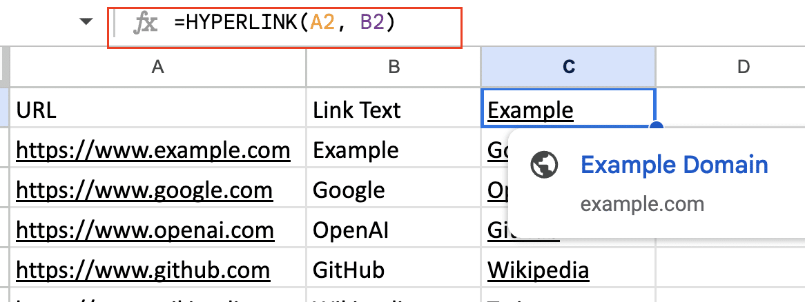
1. Using cell references for both URL and label:

=HYPERLINK(A2, B2)

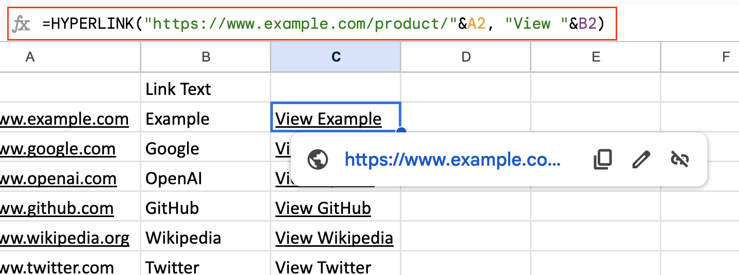
1. Combining static text with cell references:

=HYPERLINK(“https://www.example.com/product/”&A2, “View “&B2)

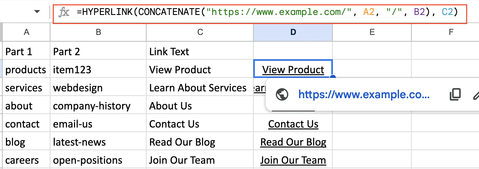
1. Using nested functions for dynamic URL generation:

=HYPERLINK(CONCATENATE(“https://www.example.com/”, A2, “/”, B2), C2)

Advanced Techniques: Combining Functions for Dynamic Hyperlinks

Using CONCATENATE with HYPERLINK

The CONCATENATE function allows you to combine multiple text strings or cell references, which is useful for creating dynamic URLs.

Example:

=HYPERLINK(CONCATENATE(“https://www.example.com/search?q=”, A2, “&category=”, B2), “Search Results”)

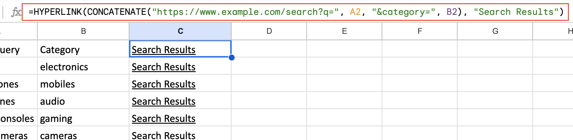
This formula creates a search URL using values from cells A2 and B2. It’s particularly useful when you need to construct complex URLs with multiple parameters.

Incorporating IF statements for conditional hyperlinks

You can use IF statements to create hyperlinks that change based on certain conditions.

Example:

=IF(A2=”In Stock”, HYPERLINK(B2, “Buy Now”), “Out of Stock”)

This formula creates a “Buy Now” link if the product is in stock, otherwise it displays “Out of Stock” without a link. You can extend this concept to create more complex conditional logic:

=IF(A2=”In Stock”, HYPERLINK(B2, “Buy Now”), IF(A2=”Pre-order”, HYPERLINK(C2, “Pre-order Now”), “Unavailable”))

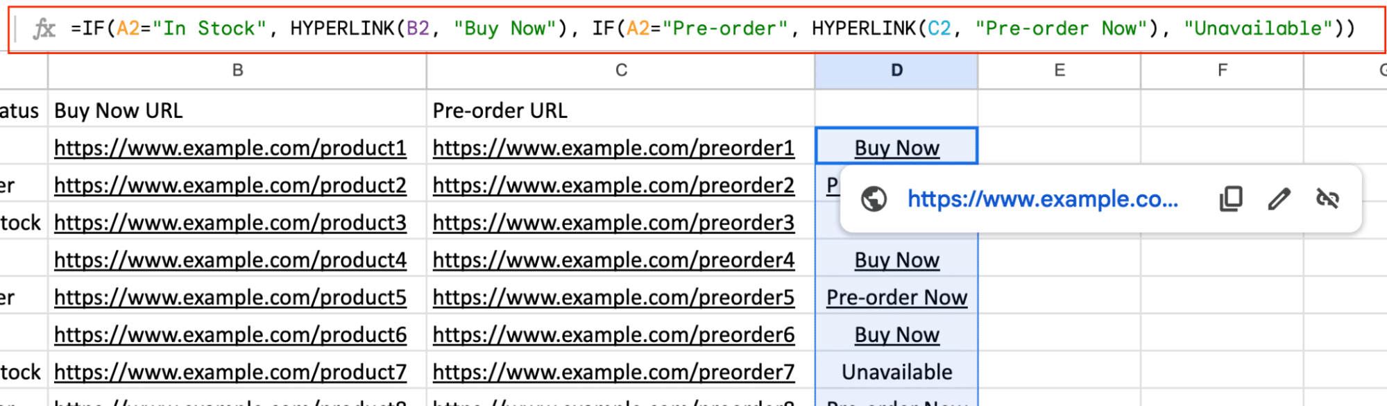
This formula adds a third option for pre-order items, demonstrating how you can chain multiple IF statements for more granular control.

Leveraging VLOOKUP for dynamic linking

VLOOKUP can be used to find specific values in a table and use them to create dynamic hyperlinks.

Example:

=HYPERLINK(VLOOKUP(A2, ProductTable, 3, FALSE), “View Product”)

This formula looks up the product code in cell A2 within a table named ProductTable and returns the URL from the third column of that table. To make this even more dynamic, you could use another cell reference for the column index:

=HYPERLINK(VLOOKUP(A2, ProductTable, B2, FALSE), VLOOKUP(A2, ProductTable, C2, FALSE))

In this case, B2 contains the column number for the URL, and C2 contains the column number for the link text, allowing for greater flexibility.

Creating Dynamic Links Between Sheets

Understanding sheet IDs and gid numbers

Each Google Sheet has a unique ID, and each tab within a sheet has a gid number. You can use these to create links between sheets or specific tabs.

To find the sheet ID, look at the URL of your Google Sheet:

https://docs.google.com/spreadsheets/d/[Sheet_ID]/edit#gid=[Tab_GID]

The Sheet ID is a long string of letters and numbers, while the gid is typically a shorter number at the end of the URL.

Formulas for linking to specific sheets and cells

To link to a specific sheet:

=HYPERLINK(“https://docs.google.com/spreadsheets/d/”&SheetID&”/edit#gid=”&TabGID, “Link Text”)

To link to a specific cell:

=HYPERLINK(“https://docs.google.com/spreadsheets/d/”&SheetID&”/edit#gid=”&TabGID&”&range=”&CellReference, “Link Text”)

Example:

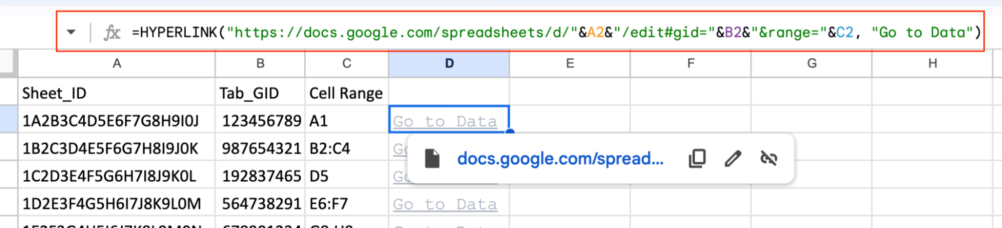
=HYPERLINK(“https://docs.google.com/spreadsheets/d/”&A2&”/edit#gid=”&B2&”&range=”&C2, “Go to Data”)

This formula creates a link using the Sheet ID from cell A2, the Tab GID from cell B2, and the cell reference from C2.

You can make this even more dynamic by using functions to generate the cell reference:

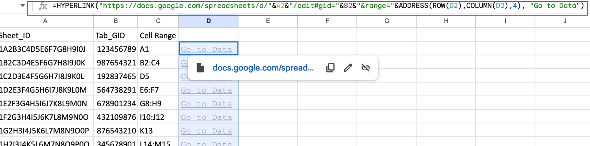
=HYPERLINK(“https://docs.google.com/spreadsheets/d/”&A2&”/edit#gid=”&B2&”&range=”&ADDRESS(ROW(D2),COLUMN(D2),4), “Go to Data”)

This formula uses the ADDRESS function to dynamically generate the cell reference based on the position of cell D2.

Best practices for organizing multi-sheet hyperlinks

1. Create a dedicated “Index” sheet with links to all other sheets.
2. Use named ranges for frequently referenced areas.
3. Implement a consistent naming convention for sheets and tabs.
4. Document your linking structure for easier maintenance.

Automating Hyperlink Creation

Using Google Sheets functions to generate multiple hyperlinks

You can use array formulas to create multiple hyperlinks at once.

Example:

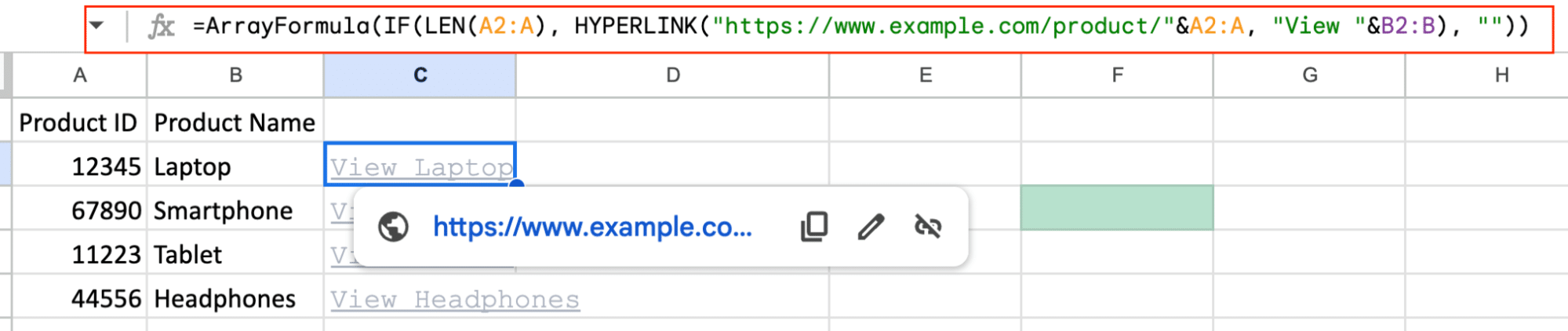
=ArrayFormula(IF(LEN(A2:A), HYPERLINK(“https://www.example.com/product/”&A2:A, “View “&B2:B), “”))

This formula creates hyperlinks for all non-empty cells in column A, using the corresponding text in column B as the link label.

You can extend this concept to create more complex automated hyperlinks:

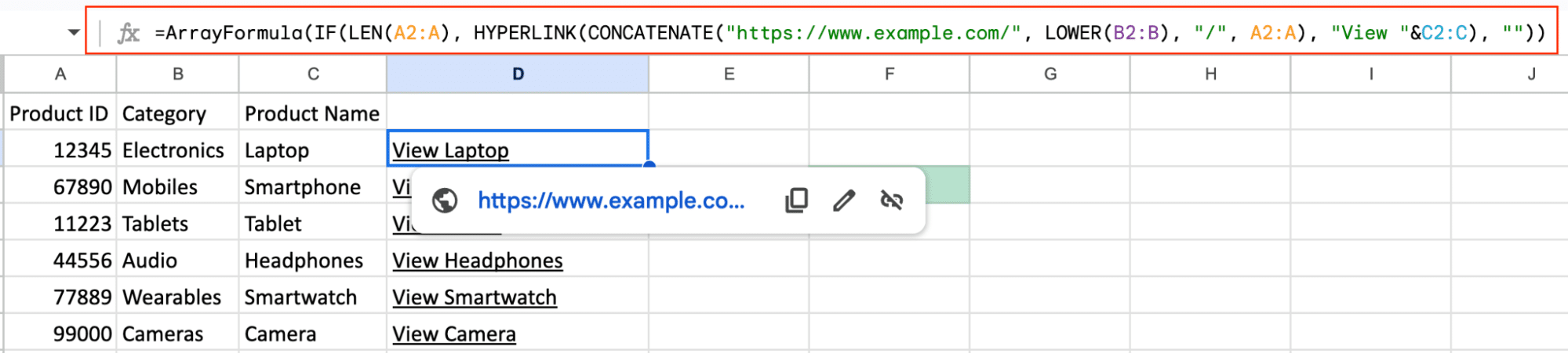
=ArrayFormula(IF(LEN(A2:A), HYPERLINK(CONCATENATE(“https://www.example.com/”, LOWER(B2:B), “/”, A2:A), “View “&C2:C), “”))

This formula combines multiple columns to create the URL and uses the LOWER function to ensure consistent formatting.

Applying custom formatting to hyperlinked cells

1. Select the cells containing your hyperlinks.
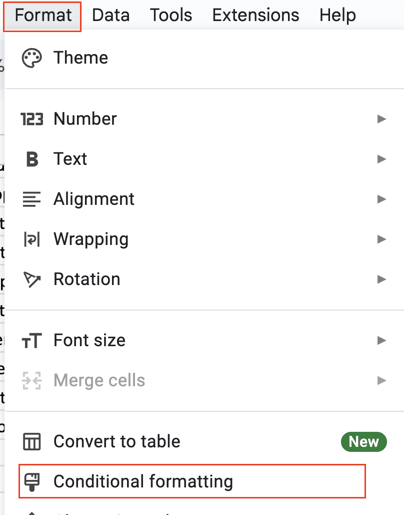
2. Click on “Format” in the menu, then “Conditional formatting.”

1. Set up a rule to apply specific formatting to cells containing hyperlinks.

Example rule: =ISURL(A2) to detect cells with hyperlinks.

You can also use custom formulas to apply different formatting based on the hyperlink content:

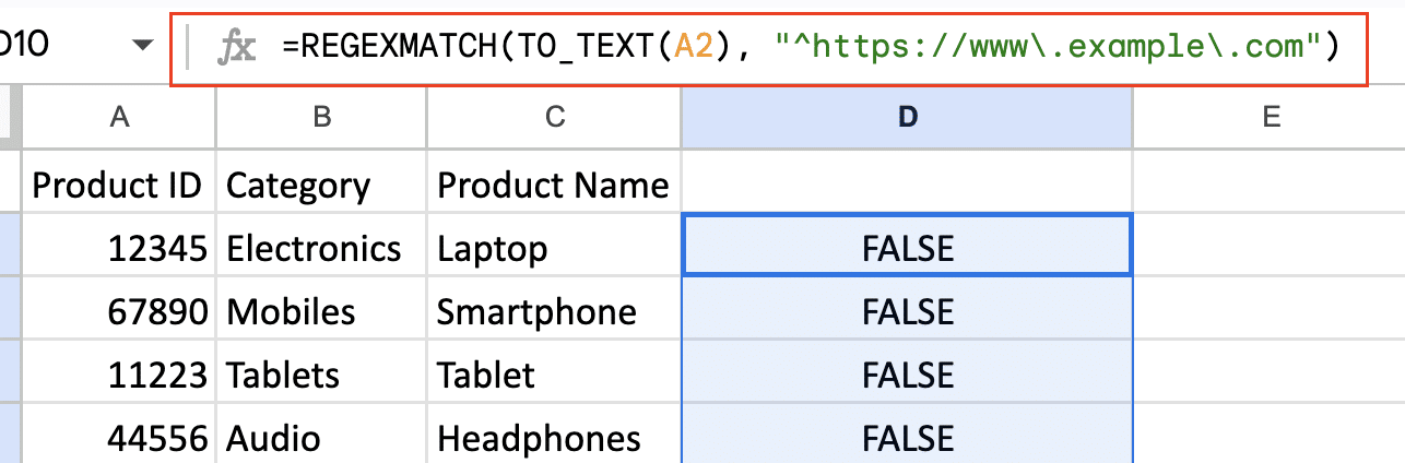
=REGEXMATCH(TO_TEXT(A1), “^https://www.example.com”)

This rule would only apply formatting to links that start with “https://www.example.com“.

Understanding Dynamic Hyperlinks in Google Sheets

What are dynamic hyperlinks?

Dynamic hyperlinks in Google Sheets are links that automatically update based on changes in your data. Unlike static hyperlinks, which remain constant, dynamic hyperlinks adapt to new information, making them incredibly useful for managing large datasets or frequently changing information.

Benefits of using dynamic hyperlinks

1. Time-saving: Eliminate the need for manual updates when your data changes.
2. Accuracy: Reduce errors associated with manual link updates.
3. Flexibility: Easily adapt your spreadsheet to new data or structures.
4. Improved user experience: Provide up-to-date, clickable links for better navigation.

Use cases and applications

Dynamic hyperlinks are valuable in various scenarios:

• Product catalogs: Link to product pages that update automatically when SKUs change.
• Employee directories: Create links to staff profiles that update with personnel changes.
• Project management: Link to task details that adjust as project statuses evolve.
• Financial reports: Generate links to specific data points that update with new financial information

By mastering these techniques for creating dynamic hyperlinks in Google Sheets, you’ll significantly enhance your spreadsheet’s functionality and efficiency. Remember to regularly review and update your hyperlinks to ensure they remain accurate and useful.

Ready to take your Google Sheets skills to the next level? Get started with Coefficient to unlock even more powerful data integration and automation features for your spreadsheets.