Applying conditional formatting to an entire row in Google Sheets is an effective way to visualize and analyze data, making it easier to identify patterns, trends, and outliers within your spreadsheet.
This method allows you to automatically highlight specific rows based on certain criteria, improving readability and making it easier to understand the data at a glance.
In this article, we will discuss how to apply conditional formatting to entire rows in Google Sheets using step-by-step instructions.
Getting to Know Conditional Formatting
Prerequisite Knowledge
Familiarity with Google Sheets, including cell, row, and column manipulation, is essential for this tutorial. Knowing how to navigate the Google Sheets interface will enhance your ability to apply conditional formatting effectively.
Definition and Use Cases
Conditional formatting in Google Sheets enables automatic cell formatting based on specific conditions. It’s ideal for:
- Highlighting sales regions exceeding targets.
- Tracking project timelines and flagging delays.
- Visualizing budget allocations and identifying overruns.
For example, a sales manager might use conditional formatting to highlight the rows of top-performing employees or to identify the orders that are pending for more than a week.
By adjusting the formatting in the cells, it becomes easier to quickly pinpoint specific information and draw meaningful conclusions.
In the next sections, we will explore how to apply conditional formatting to an entire row, making it even more convenient for users to analyze and interpret their data.
Step-by-Step Guide on Applying Conditional Formatting to Entire Row
Choosing a Condition
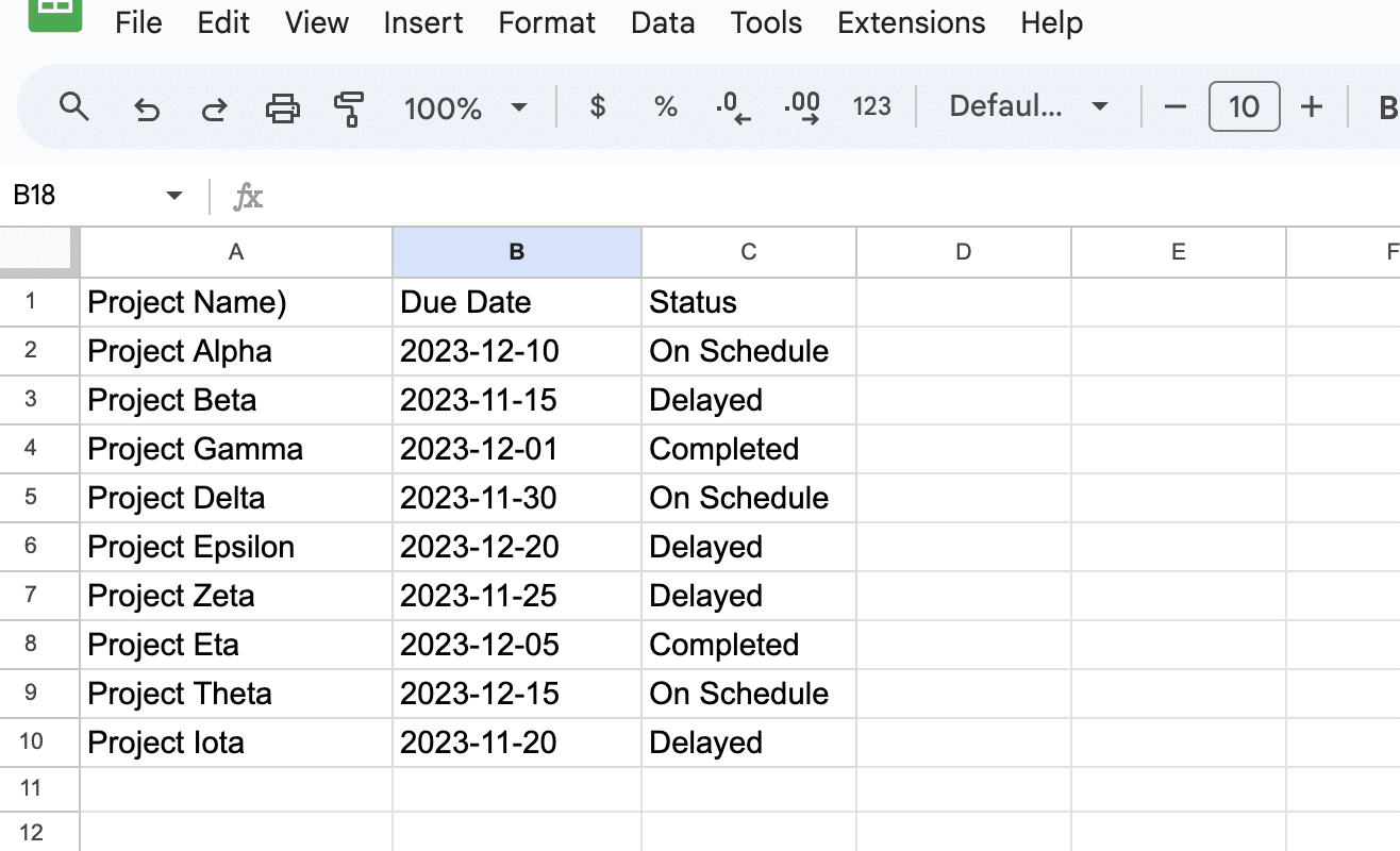
Before you start, it’s important to choose a condition based on which you want to apply conditional formatting to an entire row. Your condition could be related to a specific cell value or text in the row.
For example, you may want to identify a condition for formatting, like “Project Delayed” or “Sales Target Achieved.”
File Name: “Conditional_Formatting_Example.png”
Alt Text: “Screenshot illustrating an example of conditional formatting in Google Sheets, highlighting cells labeled ‘Project Delayed’ in red and ‘Sales Target Achieved’ in green, demonstrating how to visually identify key conditions in a dataset.”
The Formula Approach
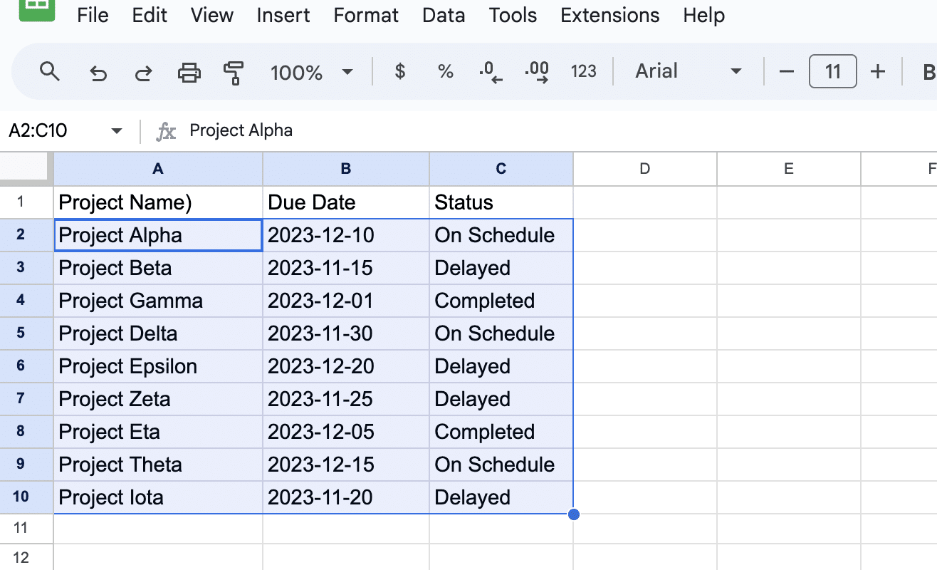
Select the range of cells where you want to apply conditional formatting. For this example, click and drag to select cells from A2 to C10.
- Screenshot:
- Filename: selecting-range-for-conditional-formatting.png
- Alt Text: Selecting the range A2:C10 in a Google Sheets project management sheet for conditional formatting.
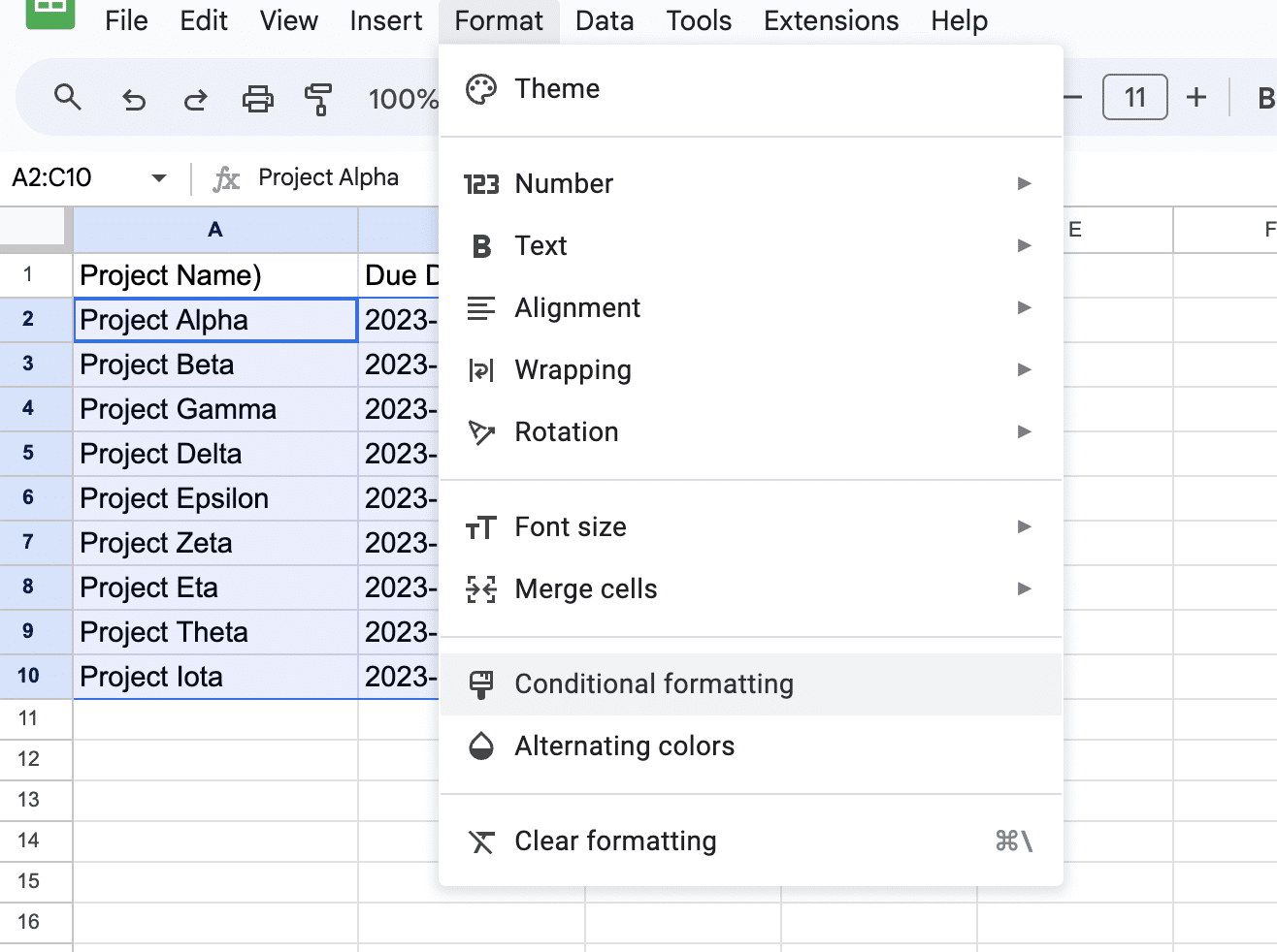
After selecting the range A2:C10, go to the menu bar.
Click on “Format”, then choose “Conditional formatting” from the dropdown menu.
- Screenshot:
- Filename: accessing-conditional-formatting-menu.png
- Alt Text: Accessing the Conditional Formatting menu in Google Sheets.
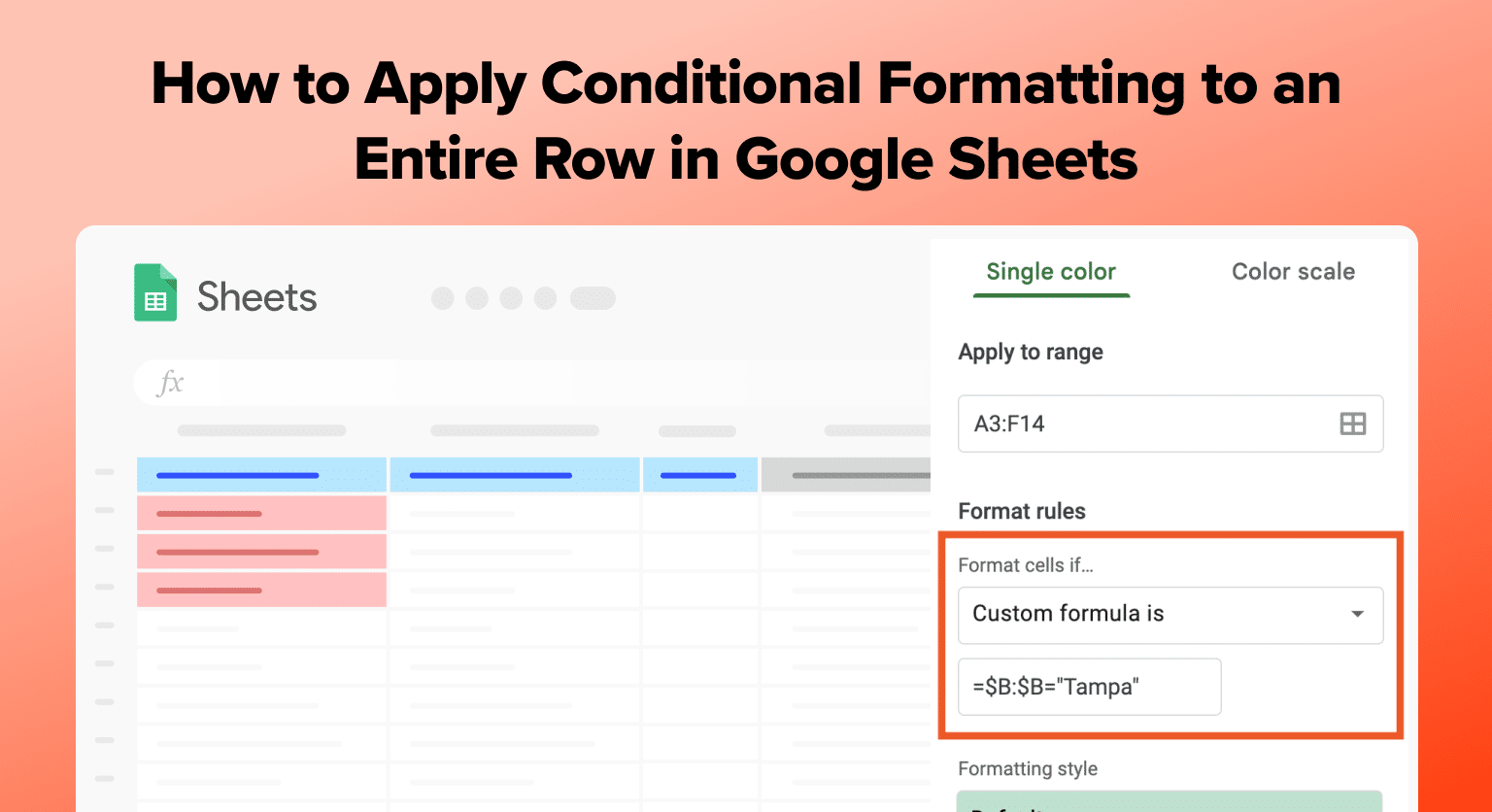
In the Conditional format rules sidebar that appears on the right, under the “Format cells if” dropdown, select “Custom formula is”.

Supercharge your spreadsheets with GPT-powered AI tools for building formulas, charts, pivots, SQL and more. Simple prompts for automatic generation.

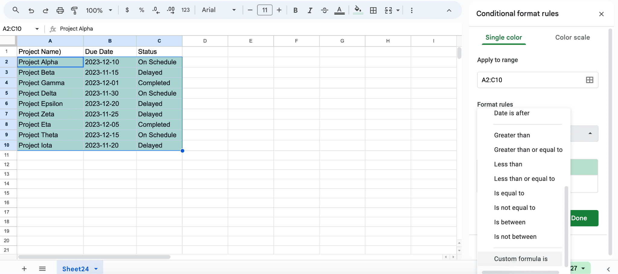
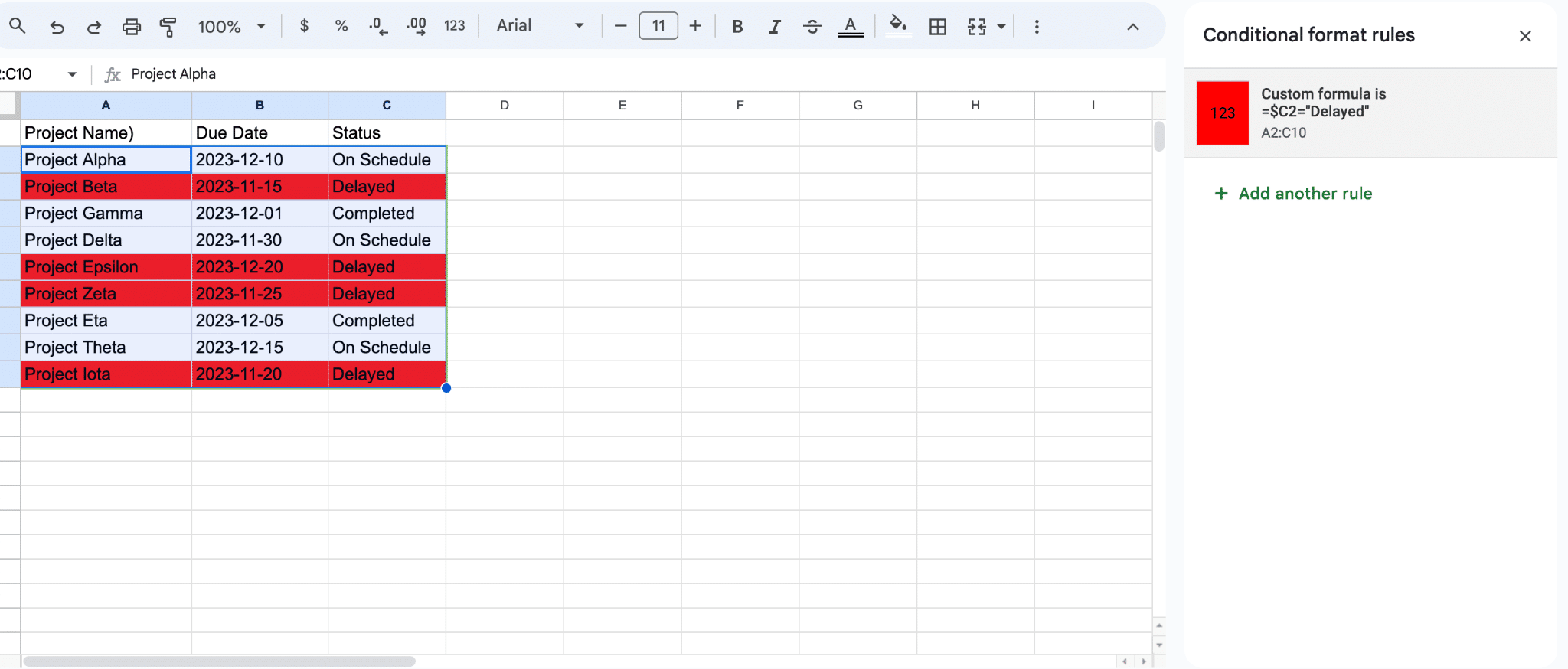
Enter the formula =$C2=”Delayed” in the box provided.
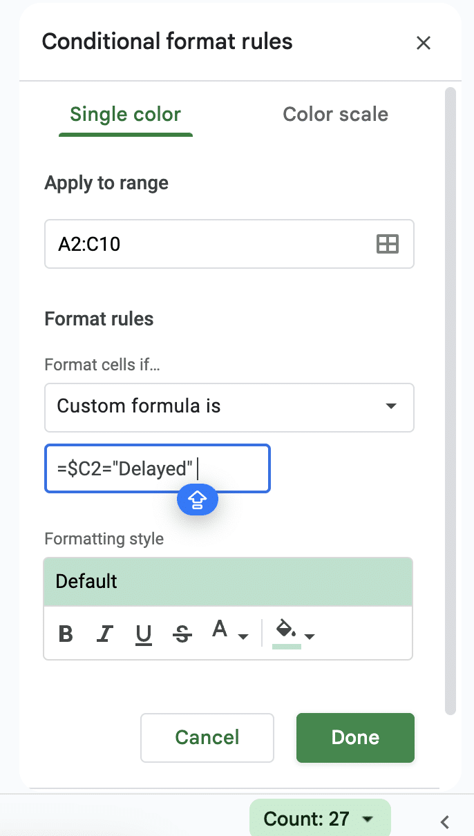
This will apply the formatting to rows where the status in column C is “Delayed”.
- Screenshot:
- Filename: setting-conditional-formatting-formula.png
- Alt Text: Setting up a conditional formatting formula in Google Sheets to highlight delayed projects.
Below the formula box, click on “Formatting style”.
File Name: “Selecting_Formatting_Style.png”
Alt Text: “Screenshot showing the selection of ‘Formatting style’ in Google Sheets, located below the formula box
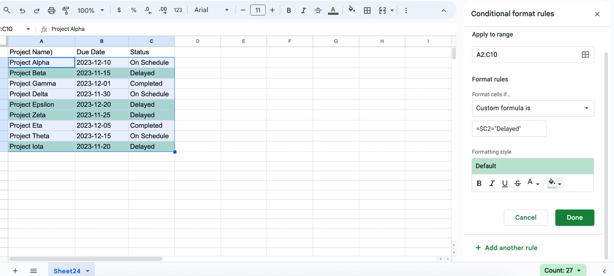
Choose a red background color to highlight the delayed projects. You can also customize the text color if desired.
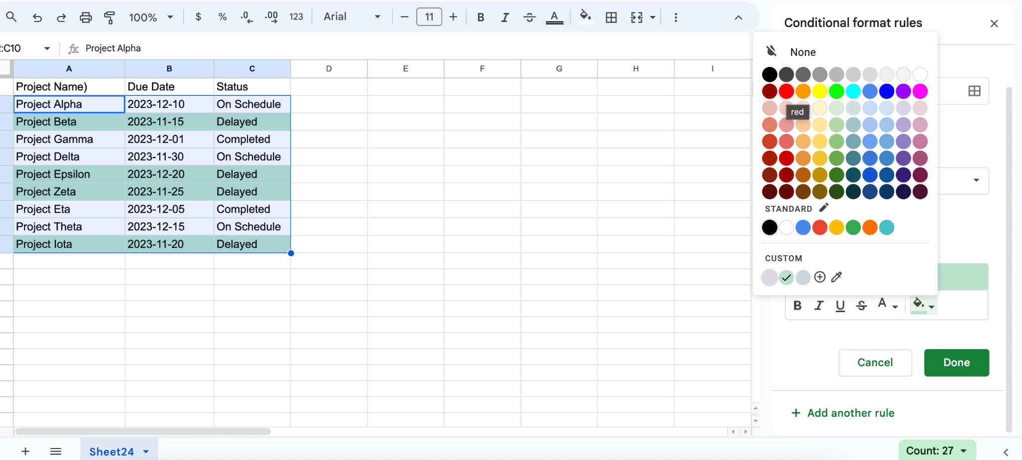
- Filename: choosing-formatting-style-conditional-formatting.png
- Alt Text: Choosing a red background as the formatting style for delayed projects in Google Sheets.
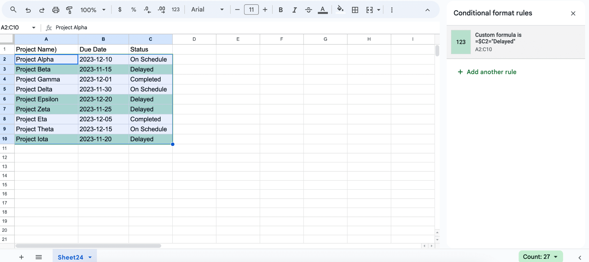
After setting up the rule and formatting style, click “Done”.
The rows where the status is “Delayed” will now be highlighted in red.
- Screenshot:
- Filename: formatted-rows-example.png
- Alt Text: Rows highlighted with conditional formatting in Google Sheets, showing delayed projects in red
Modifying or Deleting a Rule
To modify or delete an existing conditional formatting rule, Go to Format → Conditional Formatting, select the rule, and edit or delete.
Conclusion
Mastering conditional formatting in Google Sheets allows business operations teams to efficiently analyze and visualize important data. For more advanced data integration and analysis tools, consider exploring Coefficient.


