Select the cell where you want the sum to appear, then type “=SUM(” and select the range of cells you want to add
For example, to add cells A1 through A5, type “=SUM(A1
)” and press Enter
Alternatively, use manual addition by typing “=A1+A2+A3+A4+A5” with the plus sign (+) to add individual cells
The SUM function automatically updates if you change any values in the range, saving time on data changes
For conditional adding, use SUMIFS function to add values that meet specific criteria with multiple arguments
Fortunately, adding up numbers in Google Sheets is a straightforward process that can be accomplished in a variety of ways.
TLDR – The SUM function is a built-in function in Google Sheets allows you to quickly add a range of cells. To use the SUM function, simply select the cell where you want the sum to appear, type “=SUM(range of cells you want to add)”. For example, if you want to add sum of cells A1 through A5, you would type “=SUM(A1:A5)”.
Basic Summation Techniques
When working with Google Sheets, there are two basic techniques for adding numbers: using the SUM function and manual addition. Both of these techniques are simple and easy to use.
Using the SUM Function
The SUM function is a built-in function in Google Sheets that allows you to quickly add up a range of cells. To use the SUM function, simply select the cell where you want the sum to appear, type “=SUM(” and then select the range of cells that you want to add up. For example, if you want to learn how to add sum of cells in google sheets of cells A1 through A5, you would type “=SUM(A1:A5)”.
One of the advantages of using the SUM function is that it automatically updates the sum if you change any of the values in the range. This can save you a lot of time if you need to make changes to your data.
Manual Addition
Manual addition is another simple technique for adding numbers in Google Sheets. To use manual addition, simply select the cell where you want the sum to appear and then type the formula using the plus sign (+) to add up the values. For example, if you want to add up the values in cells A1 through A5, you would type “=A1+A2+A3+A4+A5”.
While manual addition may take more time than using the SUM function, it can be useful if you only need to add up a small number of values or if you want to perform other calculations in the same formula.
Advanced Summation Methods
Summing Across Sheets
In some cases, you may have data spread across multiple sheets in the same Google Sheets file. To add up the values from these sheets, you can use the SUM function with the sheet name and cell range specified. For example, to add up the values in cell A1 from Sheet1 and cell A1 from Sheet2, you would use the following formula:
=SUM(Sheet1!A1, Sheet2!A1)
You can also use the SUM function with a named range that spans multiple sheets. To create a named range, select the cells you want to include and click “Data” > “Named ranges”. Give the range a name and select the sheets you want to include. Then, you can use the named range in the SUM function. For example, if you named a range “MyRange” that includes cells A1 through A5 on Sheet1 and Sheet2, you would use the following formula to add up the values:
=SUM(MyRange)
Conditional Sums with SUMIF
Sometimes, you may only want to add up values that meet certain criteria. In this case, you can use the SUMIF function. The SUMIF function takes three arguments: the range to check, the criteria to check for, and the range to sum. For example, if you wanted to add up all the values in column A that are greater than 10, you would use the following formula:
=SUMIF(A:A, “>10”)
You can also use the SUMIF function to add up values based on multiple criteria. For example, if you wanted to add up all the values in column A that are greater than 10 and less than 20, you would use the following formula:

Supercharge your spreadsheets with GPT-powered AI tools for building formulas, charts, pivots, SQL and more. Simple prompts for automatic generation.

=SUMIFS(A:A, A:A, “>10”, A:A, “<20”)
The SUMIFS function takes multiple arguments: the range to sum, the range to check for the first criteria, the first criteria, the range to check for the second criteria, and the second criteria. You can add more criteria by adding additional pairs of ranges and criteria.
In conclusion, Google Sheets offers many simple and advanced summation methods to help you add up values in your spreadsheets. Use these techniques now to save time and get more accurate results.
Leverage AI to Build Your Google Sheets Formulas
There are over 500 Google Sheets functions that exist today, which make almost anything you can dream up possible in Google Sheets. And, spreadsheet skills are useful for almost any profession. However, it takes time to master formulas and functions. A simple way to get ahead? You can use Coefficient’s free Formula Builder to automatically create your Google Sheets formulas, pivots, and charts for you.
First, you’ll need to install the free Google Sheets Extension. You can get started with Formula Builder here.
After you submit your email, follow along, and accept the prompts to install. Once the installation is finished, navigate to Extensions on the Google Sheets menu. Coefficient will be available as an add-on.
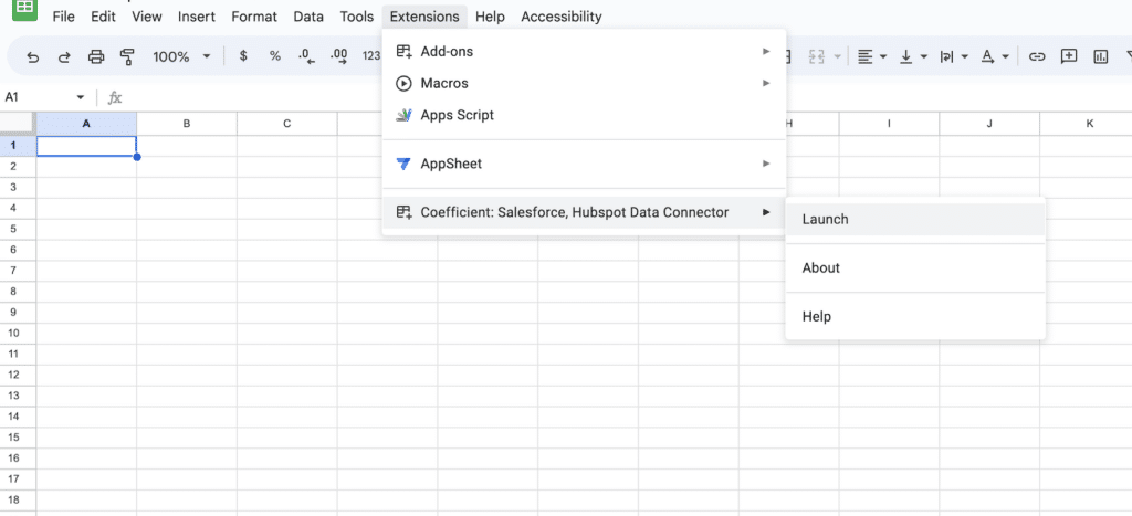
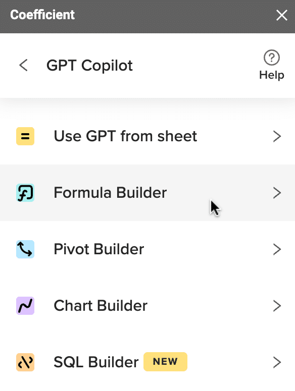
Now launch the app. Coefficient will run on the sidebar of your Google Sheet. Select GPT Copilot on the Coefficient sidebar.

Then click Formula Builder.
Type a description of a formula into the text box. For this example, let’s sort 20 dates starting with the most recent date.
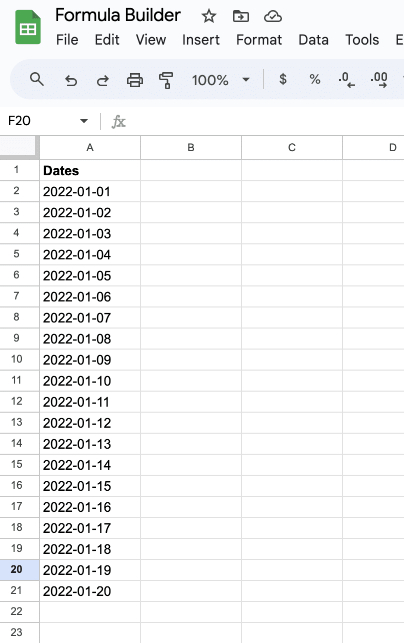
Simply type: Sort dates in column A in sheet9 by most recent date.
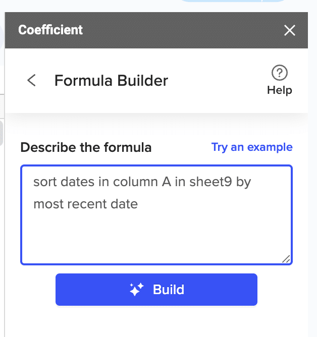
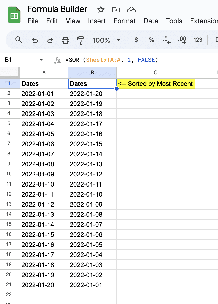
Then press ‘Build’. Formula Builder will automatically generate your sort formula.
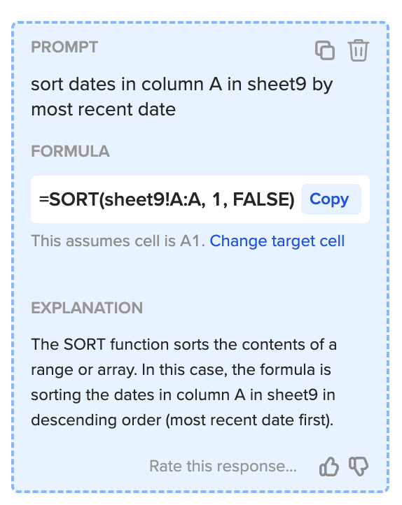
And, it’s that easy! Simply, place the formula in the desired cell.
