Mastering SQL in Google Sheets: The Ultimate Guide to Powerful Data Analysis

Are you struggling to analyze large datasets in Google Sheets? Do you wish you could leverage the power of SQL without leaving your spreadsheet? This comprehensive guide will teach you how to use SQL-like queries in Google Sheets, transforming your spreadsheet into a robust data analysis tool.

Getting Started with Google Sheets SQL

Setting up your data

Before you can start using SQL-like queries in Google Sheets, you need to ensure your data is properly structured:

1. Organize your data in a tabular format
2. Include headers in the first row
3. Ensure consistent data types within each column
4. Remove any blank rows or columns

Basic syntax of the QUERY function

The QUERY function in Google Sheets follows this basic structure:

=QUERY(data_range, “SELECT … WHERE … GROUP BY … ORDER BY …”, [headers])

Let’s break down each component:

• data_range: The range of cells containing your data
• “SELECT … WHERE … GROUP BY … ORDER BY …”: The SQL-like query string
• [headers]: An optional parameter specifying the number of header rows (default is 1)

Understanding Google Sheets Query Language (GQL)

Google Sheets Query Language (GQL) is the SQL-like language used within the QUERY function. While similar to SQL, it has some unique features and limitations:

1. Case-insensitive keywords (e.g., SELECT, WHERE, ORDER BY)
2. Column references use letters (A, B, C) instead of names
3. Limited set of functions compared to full SQL
4. Some syntax differences (e.g., using CONTAINS instead of LIKE)

Essential SQL-like Operations in Google Sheets

SELECT: Choosing specific columns

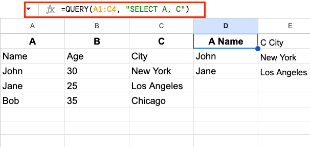
The SELECT clause allows you to specify which columns you want to include in your query results.

A	B	C
Name	Age	City
John	30	New York
Jane	25	Los Angeles
Bob	35	Chicago

=QUERY(A1:C4, “SELECT A, C”)

Name	City
John	New York
Jane	Los Angeles
Bob	Chicago

WHERE: Filtering data

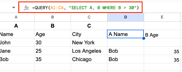
The WHERE clause allows you to filter your data based on specific conditions.

A	B	C
Name	Age	City
John	30	New York
Jane	25	Los Angeles
Bob	35	Chicago

=QUERY(A1:C4, “SELECT A, B WHERE B > 30”)

Name	Age
Bob	35

ORDER BY: Sorting results

The ORDER BY clause allows you to sort your query results based on one or more columns.

A	B	C
Name	Age	City
John	30	New York
Jane	25	Los Angeles
Bob	35	Chicago

=QUERY(A1:C4, “SELECT A, B, C ORDER BY B DESC”)

Name	Age	City
Bob	35	Chicago
John	30	New York
Jane	25	Los Angeles

GROUP BY: Aggregating data

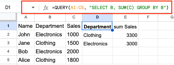
The GROUP BY clause allows you to group rows that have the same values in specified columns.

A	B	C
Name	Department	Sales
John	Electronics	1000
Jane	Clothing	1500
Bob	Electronics	2000
Alice	Clothing	1800

=QUERY(A1:C5, “SELECT B, SUM(C) GROUP BY B”)

Department	SUM of Sales
Electronics	3000
Clothing	3300

LIMIT: Restricting the number of results

The LIMIT clause allows you to specify the maximum number of rows to return in your query results.

A	B	C
Name	Age	City
John	30	New York
Jane	25	Los Angeles
Bob	35	Chicago
Alice	28	Boston

=QUERY(A1:C5, “SELECT A, B, C ORDER BY B DESC LIMIT 2”)

Name	Age	City
Bob	35	Chicago
John	30	New York

Advanced QUERY Techniques

JOINing data from multiple sheets

While Google Sheets doesn’t support traditional SQL JOINs, you can simulate JOIN operations using the QUERY function in combination with other functions like VLOOKUP or ARRAYFORMULA.

Sheet1:

A	B
ID	Name
1	John
2	Jane
3	Bob

Sheet2:

A	B
ID	Salary
1	50000
2	60000
3	55000

Query (in a new sheet):

=QUERY({Sheet1!A:B, ARRAYFORMULA(VLOOKUP(Sheet1!A:A, Sheet2!A:B, 2, FALSE))},

“SELECT Col1, Col2, Col3 WHERE Col3 IS NOT NULL”)

ID	Name	Salary
1	John	50000
2	Jane	60000
3	Bob	55000

Using aggregate functions (SUM, AVG, COUNT, etc.)

Google Sheets QUERY supports various aggregate functions that allow you to perform calculations on groups of rows.

A	B	C
Name	Department	Sales
John	Electronics	1000
Jane	Clothing	1500
Bob	Electronics	2000
Alice	Clothing	1800

=QUERY(A1:C5, “SELECT B, SUM(C), AVG(C), COUNT(A) GROUP BY B”)

Department	SUM of Sales	AVG of Sales	COUNT of Name
Electronics	3000	1500	2
Clothing	3300	1650	2

Creating pivot tables with QUERY

The QUERY function can be used to create pivot table-like results directly in your spreadsheet.

A	B	C	D
Date	Product	Category	Sales
2023-01-01	Widget A	Electronics	1000
2023-01-02	Gadget B	Appliances	1500
2023-01-03	Widget C	Electronics	2000
2023-01-04	Gadget D	Appliances	1800

=QUERY(A1:D5, “SELECT C, SUM(D) GROUP BY C PIVOT B”)

Category	Widget A	Gadget B	Widget C	Gadget D
Electronics	1000		2000
Appliances		1500		1800

Handling date and time data

Google Sheets QUERY provides several functions for working with date and time data.

A	B	C
Date	Event	Attendees
2023-01-01	New Year’s Party	100
2023-02-14	Valentine’s Day	50
2023-03-17	St. Patrick’s Day	75
2023-04-01	April Fool’s Day	25

=QUERY(A1:C5, “SELECT MONTH(A), SUM(C) GROUP BY MONTH(A) LABEL MONTH(A) ‘Month'”)

Month	SUM of Attendees
1	100
2	50
3	75
4	25

Real-world Applications and Use Cases

Financial analysis and reporting

Use SQL-like queries in Google Sheets to analyze financial data, calculate key metrics, and generate reports.

A	B	C	D
Date	Category	Income	Expenses
2023-01-01	Salary	5000
2023-01-05	Rent		1500
2023-01-10	Groceries		300
2023-01-15	Freelance	1000

=QUERY(A1:D5, “SELECT SUM(C), SUM(D) LABEL SUM(C) ‘Income’, SUM(D) ‘Expenses'”)

Category	Income	Expenses	Net Income
Total	6000	1800	4200

Marketing campaign performance tracking

Evaluate the effectiveness of marketing campaigns by analyzing key performance indicators.

A	B	C	D	E
Date	Campaign	Impressions	Clicks	Conversions
2023-01-01	Email	10000	500	50
2023-01-02	Social Media	50000	1000	75
2023-01-03	PPC	25000	750	60
2023-01-04	Email	15000	600	55

=QUERY(A1:E5, “SELECT B, SUM(C), SUM(D), SUM(E), SUM(D) / SUM(C) * 100, SUM(E) / SUM(D) * 100 GROUP BY B ORDER BY SUM(E) DESC”)

Campaign	Impressions	Clicks	Conversions	CTR (%)	Conversion Rate (%)
Social Media	50000	1000	75	2.00	7.50
PPC	25000	750	60	3.00	8.00
Email	25000	1100	105	4.40	9.55

Tips and Best Practices for Google Sheets SQL

Optimizing QUERY performance

1. Limit the data range to only necessary columns and rows
2. Use appropriate data types for each column
3. Avoid unnecessary calculations within the query
4. Use LIMIT clause when working with large datasets
5. Consider using VLOOKUP or INDEX/MATCH for simple lookups instead of QUERY

Handling errors and troubleshooting

Common errors and solutions:

1. “Unable to parse query string”: Check for syntax errors in your query
2. “No column X”: Ensure column references are correct (A, B, C, etc.)
3. “Circular dependency”: Avoid referencing the query result within the query itself
4. “Mismatched data types”: Ensure consistent data types within columns

Combining QUERY with other Google Sheets functions

Enhance your queries by combining QUERY with other functions:

1. Use ARRAYFORMULA for array operations
2. Incorporate VLOOKUP or INDEX/MATCH for joining data
3. Utilize TEXT functions for string manipulation
4. Leverage DATE functions for date-based calculations

=QUERY({A1:C10, ARRAYFORMULA(IF(B1:B10>30, “Senior”, “Junior”))},

“SELECT Col1, Col2, Col3, Col4 WHERE Col4 = ‘Senior'”)

Google Sheets SQL? Use Coefficient.

By mastering SQL-like queries in Google Sheets and leveraging external connections, you can transform your spreadsheets into powerful data analysis tools. Start experimenting with these techniques today to unlock new insights from your data!

Ready to take your data analysis to the next level? Get started with Coefficient and connect your Google Sheets to powerful SQL databases for seamless data integration and advanced analytics.