
What Is XLOOKUP?
XLOOKUP Excel is a function developed to look for data in a table or range and return the corresponding value. It replaces older functions like VLOOKUP and HLOOKUP by providing more convenience and effectiveness. With its ability to perform lookups regardless of the table’s layout or size, XLOOKUP significantly simplifies formula writing and reduces errors, making it a favorite among Excel users.
XLOOKUP does vertical and horizontal lookups without needing fixed column settings or binary search. This function provides the same matching and exact matching and supports search in any direction, increasing the user’s efficiency and improving data handling.
XLookup Compared With Other Functions
XLookup vs VLookup vs HLookup
XLOOKUP is a bidirectional function that enables vertical and horizontal search, facilitating more flexible data lookups. It can return arrays, making it useful for complex calculations. XLOOKUP Excel also supports wildcard characters for partial matches, enhancing its utility in scenarios where exact data entries are unknown.
This feature is particularly advantageous for managing large datasets with varying details. Importantly, XLOOKUP treats missing values with precision by providing a facility to create custom messages when not found. Its power to work with unsorted data will save time and result in high efficiency, making XLOOKUP a better and more robust alternative to Excel. Here’s a comparison table for better understanding.
| Feature | XLOOKUP | VLOOKUP | HLOOKUP |
| Search Direction | Any direction | Vertical only | Horizontal only |
| Column Index Requirement | No | Yes | Yes |
| Handling of Missing Values | Customizable return values | Returns error if not found | Returns error if not found |
| Works on Unsorted Data | Yes | No (sorted data required for approximate match) | No (sorted data required for approximate match) |
| Return Arrays | Yes | No | No |
| Flexibility | High (can replace both VLOOKUP and HLOOKUP) | Moderate | Moderate |
XLOOKUP stands out as a more up-to-date and adaptable function compared to VLOOKUP and HLOOKUP. Its capability to manage both horizontal and vertical lookups, handle missing values cautiously, operate with primitive data, and return arrays makes it a significant tool for professionals in marketing, finance, and Data/Bi.
XLOOKUP Excel Formula
The XLOOKUP function in Excel represents an efficient way to search and extract data. Here is the function syntax followed by a detailed breakdown of each parameter, including examples:
=XLOOKUP(lookup_value, lookup_array, return_array, [if_not_found], [match_mode], [search_mode])
The formula consists of several components that work together to perform the desired lookup. Let’s understand each component in detail:
- Lookup_value – This is the value you are searching for within the lookup_array. For example, if you want to find the salary of an employee named “John,” “John” would be your lookup_value.
- Lookup_array – This is the range of cells containing the data you are searching. In the previous example, this would be the column containing employee names.
- Return_array – This range contains the data you want to retrieve. For example, if you are looking up “John’s” salary, the return_array column would contain salaries.
- If_not_found (optional) – You can specify what should return if the lookup_value is not found in the lookup_array. For example, you might have “Not Found” as the return value if “John” isn’t listed in the employee column.
- Match_mode (optional) –
- 0: Returns an exact match. If no exact match is found, it results in an error unless an if_not_found value is specified.
- -1: Finds the smallest value greater than or equal to lookup_value.
- 1: Find the most significant value that is less than or equal to lookup_value.
- 2: Allows for wildcard characters, such as ‘?’ (to replace a single character) or ‘ * ’ (to replace any sequence of characters). For example, if your lookup_value is “Jo*,” it would match “John,” “Joan,” etc.
- Search_mode (optional) –
- 1: Searches from the beginning of the lookup_array to the end.
- -1: Searches from the end of the lookup_array to the beginning are useful for finding the last occurrence of the lookup_value.
- 2: Uses a binary search to find the first value equal to the lookup_value in an ascending-sorted lookup_array. This is faster but requires the array to be sorted.
- -2: Similar to 2 but used for descending-sorted arrays.
Example Formula:
=XLOOKUP(A2, B2:B10, C2:C10, “Not found”, 0, 1)
In this formula:
1. A2 is the cell containing the employee name we want to search for.
2. B2:B10 is the range of cells containing employee names.
3. C2:C10 is the range of cells containing employee salaries, aligned with the names in B2:B10.
4. “Not found” specifies what to return if the employee name in A2 is not found in the range B2:B10.
5. 0 indicates that we want an exact match of the employee name.
6. 1 directs the function to search from the first to the last entry (top to bottom) in the lookup array.
Essential Precautions to Know Before Using XLOOKUP in Excel
Before the Step-by-Step Tutorial of XLOOKUP, it’s crucial to understand the precautions to ensure smooth and accurate data retrieval. By identifying typical mistakes and sharing recommended practices, users can utilize the dynamic feature of this Excel function to the full extent.
- Ensure Data Consistency: Verify that the lookup and return arrays align with the consistent data type to avoid any mismatch.
- Handle #N/A Errors: Use the ‘iferror’ function with XLOOKUP to deal with instances of no match.
- Define Search Mode: State the search mode precisely. It will control the search direction and match type and exclude unexpected results.
- Use Absolute References: When copy-pasting formulas, use absolute cell references instead of relative ones so that the array references remain valid.
- Avoid Volatile Dependencies: Make sure that XLOOKUP’s dependency is not too volatile; otherwise, the workbook’s performance will be much slower.
By following these precautions, users can leverage the full potential of this powerful Excel function for accurate and efficient data retrieval.
Video Tutorial
Check out the tutorial below for a complete video walkthrough!
How To Use the XLOOKUP Function in Excel?
Step 1: Select the cell for XLOOKUP
First, you need to choose the correct cell in the Excel worksheet where the XLOOKUP output will be generated. This is your output cell, where you will see the data that was retrieved after the function completes its execution successfully. Data integrity must be considered to ensure that the output does not interfere with other data in your worksheet and does not disrupt the existing formulas or data structures.
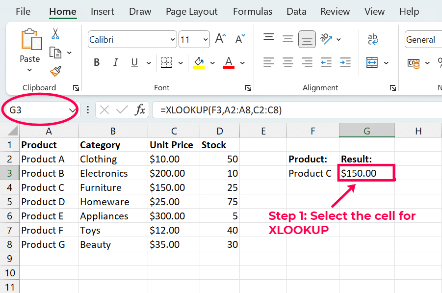
For example, if you want to find the unit price of “Product C,” you can simply enter the product name in the search bar, and you will be provided with the relevant information. Here, I have placed it in a cell that is easy to view, such as cell G3, which is near the data table.
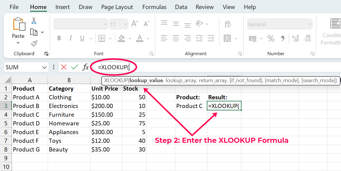
Step 2: Enter the XLOOKUP Formula
Click on the selected cell and begin to type your formula. Start with “=XLOOKUP(“.
Step 3: Add the Lookup Value
The first parameter in the XLOOKUP function is the “lookup_value.” You want Excel to search for this value in the lookup array. The lookup value must be defined accurately to retrieve the correct data.
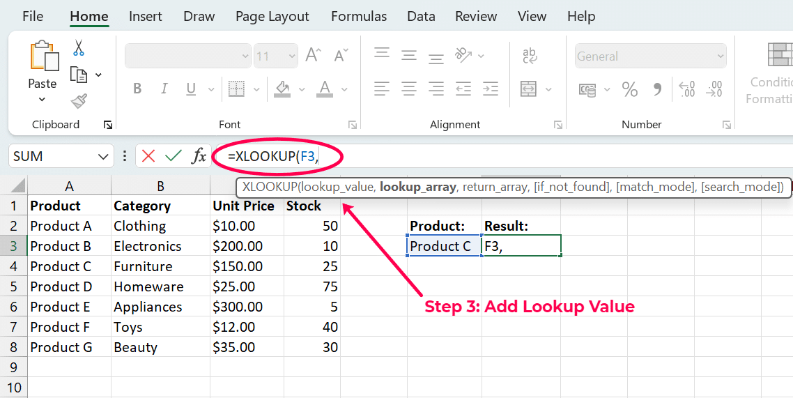
For example, if you are searching for the price of “Product C,” your lookup value will be “Product C.” You could also add “Product C” in another cell and add the cell value, which is “F3.” In your formula bar, it would look like this: “=XLOOKUP(F3,“.

Stop exporting data manually. Sync data from your business systems into Google Sheets or Excel with Coefficient and set it on a refresh schedule.
Get Started
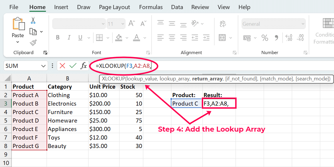
Step 4: Add the Lookup Array
The ‘lookup_array’ is the range where Excel will look for the ‘lookup_value.’ It should be a column or row with the value you’re trying to match. In our example, if “Product C” and other product names are listed in column A from cell A2 to A8, you would set A2:A8 as your lookup array.
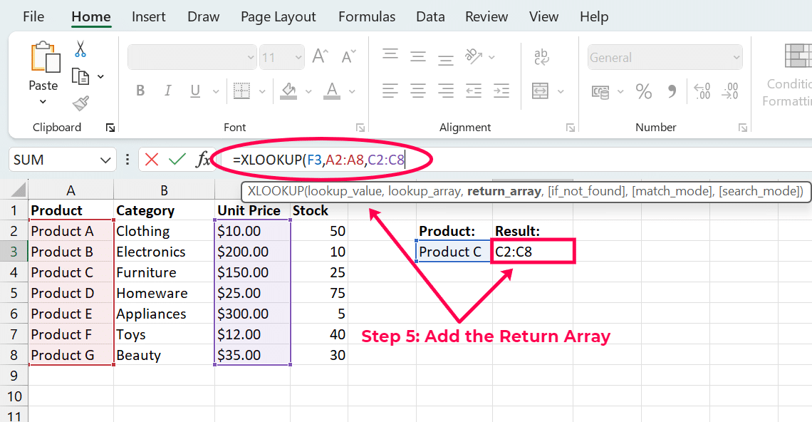
Step 5: Specify the Column Index Number
The ‘return_array’ is the range from which Excel will pull the data you want to retrieve once it finds a match for the lookup value in the lookup array. This should be in the same row or column orientation as your lookup array. Continuing our example, if unit prices are in column C from cells C2 to C8, then your return array would be C2:C8.
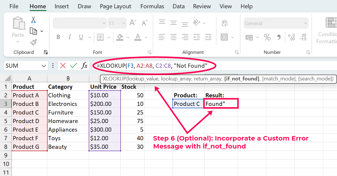
Step 6 (Optional): Incorporate a Custom Error Message with if_not_found
This optional parameter lets you define what should be displayed if the ‘lookup_value’ is not found in the ‘lookup_array.’ This can be particularly useful for error handling and ensuring that your data presentation remains clean and understandable. In your formula bar, it would look like this: “=XLOOKUP(F3, A2:A8, C2:C8, “Not Found”,“.
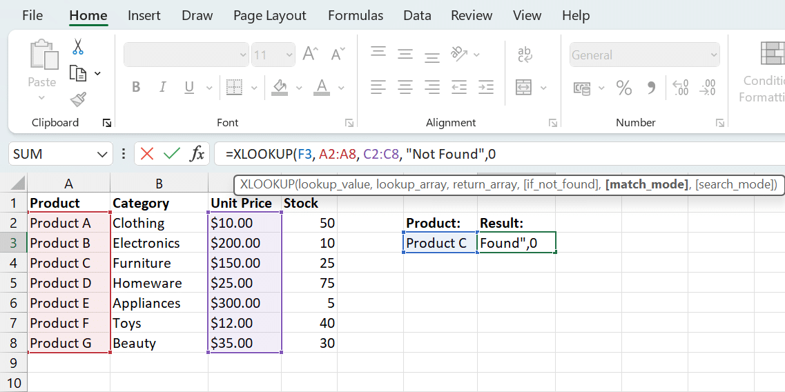
Step 7 (Optional): Tailor Your Search with match_mode Options
The ‘match_mode’ parameter lets you specify how Excel matches the ‘lookup_value’ with values in the ‘lookup_array’. You can set this parameter to ‘0’ for an exact match, ‘-1’ for an exact match or next smallest, ‘1’ for an exact match or next more significant, and ‘2’ for a wildcard match. The formula would be “=XLOOKUP(F3, A2:A8, C2:C8, “Not Found”, 0“.
Step 8 (Optional): Adjust Search Direction and Order with search_mode
The search_mode parameter allows you to define the direction of the search. ‘1’ is for a search that starts at the first item and moves forward, while ‘-1’ is for a search that begins at the last item and moves backward.
Final Formula “=XLOOKUP(F3, A2:A8, C2:C8, “Not Found”, 0, 1)”
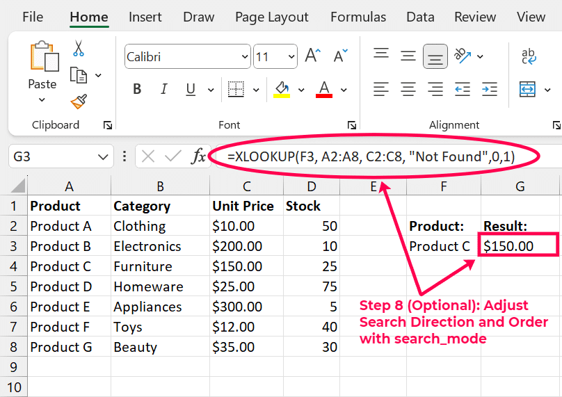
Press Enter after typing the complete formula to execute the XLOOKUP and see the result in the selected cell. This robust function makes data retrieval efficient and ensures that your spreadsheets are more dynamic and responsive to data changes.
How XLOOKUP Is Useful For Professionals In Marketing, Finance, Data/BI
The XLOOKUP Excel Function is a significant tool for professionals across numerous fields, giving substantial benefits in tasks regarding marketing, finance and data/business intelligence (BI). Here’s how it can be helpful in each of these domains:
Marketing
- Customer Data Management – Marketing specialists can utilize XLOOKUP to rapidly locate customer information across large datasets. For example, recovering the e-mail addresses of customers based on customer IDs from a list.
- Campaign Analysis – XLOOKUP helps in consolidating campaign performance information from various sources, enabling a pragmatic analysis. You can simply pull in metrics like click-through rates or altering rates by the name of the campaign.
- Segmentation – It supports customer segmentation by complementing demographic information with behavioral data, making it easier to quarry precise groups with tailored marketing plans.
Finance
- Financial Reporting – XLOOKUP streamlines the process of pulling precise financial data from comprehensive financial reports. For instance, you can extract periodic revenue figures for a precise department.
- Budget Tracking – Finance specialists can use XLOOKUP to contrast budgeted expenses with true expenses, simplifying contention analysis.
- Investment Analysis – It aids in captivating historical stock prices or financial metrics for precise firms, which is crucial for building investment models and yielding trend analysis.
Data/Business Intelligence (BI)
- Data Consolidation – In Business Intelligence, XLOOKUP can be used to amalgamate data from distinct tables or databases. This is critical for creating combined reports that offer applicable insights.
- Real-Time Dashboards – Bi specialists can use XLOOKUP to create lively dashboards. For example, pulling the newest sales data based on product IDs to exhibit in real-time reports.
- Error Handling – The function’s capability to manage errors cautiously with the [if_not_found] argument ensures data incorporation and credibility in reports.
Pro Tips To Improve Your XLOOKUP Skills
Expert Advice for Optimizing Performance:
- Minimize Lookup Range: Narrow down the lookup array to its most essential range. This minimizes the data volume and hence speeds up the calculation processes.
- Use Exact Matches: By default, use exact matches (match_mode set to 0) because they are more performance-friendly than approximate matches.
- Avoid Volatile Dependencies: Try to ensure that the cells referenced in the XLOOKUP function are not volatile (i.e., not subject to frequent updates), as this can slow down performance through many recalculations.
Creative Uses of XLOOKUP in Complex Excel Projects:
- Data Merge: Employ XLOOKUP to consolidate data from different sheets or tables based on a shared index, such as connecting to the sales data of customers where the customer ID is the connecting key.
- Two-way Lookup: Combine horizontal and vertical lookups vertically by nesting XLOOKUP functions. This lets you move across rows and down the columns to a specific place in the table to find a value.
- Conditional Formatting Helper: Apply XLOOKUP to locate the criteria or formats based on specific criteria. Thus, the sheet is automatically formatted based on the retrieved values from the other table.
Advanced XLOOKUP Features and Applications
Integrating XLOOKUP Excel with Other Functions for Advanced Analysis:
- With TEXTJOIN: Combine XLOOKUP with TEXTJOIN, to sum up text data depending on a criterion from different sheets or tables.
- With SUMIFS: Apply XLOOKUP to grab a dynamic range for your criteria in SUMIFS, and the summation will be based on dynamic criteria.
- Sequential Lookups: Chain the XLOOKUPs to perform sequential lookups, where the output of one XLOOKUP becomes the input of the next one.
Applications Where the XLOOKUP Feature Can Be Used:
- Financial Modeling: They are convenient for pulling financial data into models based on dates or other identifiers.
- Inventory Management: Searching for inventory levels or locations using item codes is easy and quick.
- HR Data Handling: It is used in situations where data needs to be fetched across multiple sheets, such as payroll, leave records, and performance appraisals, using employee IDs.
Common Errors and Troubleshooting XLOOKUP
Identify and Resolve Typical Errors:
- #N/A Errors: Usually, the outcome is that the lookup value is not available in the lookup array. Verify the existence of the value or put an if_not_found parameter in place in case of missing values to deal with the situation smoothly.
- #VALUE! Errors: Check if the lookup value and array data types match (e.g., text vs. number mismatches).
- Reference Errors: Ensure that the lookup and return arrays are appropriately aligned and that you are not accidentally referencing cells outside the intended range.
Using The XLOOKUP Excel Function
In this article, we did a deep dive into how the XLOOKUP Excel function works and discussed some advanced functions too. This function is especially useful when working with real-time data.
But how do you bridge the gap between your external databases and Excel sheets where you’re doing data analysis?
Introducing Coefficient, which ensures data accuracy and eliminates the need for manual updates. The tool’s robust connectors facilitate direct data pulls from platforms such as Salesforce and SQL Server into Excel, making it possible to apply XLOOKUP seamlessly on the latest data. Users benefit from automatic refreshes that keep data current, enhancing the reliability of lookup functions. Get started with Coefficient today!


