The WRAPCOLS function, new in Excel 2025, converts linear data into organized columns. It’s the solution when you need to display long lists in a more readable format. Whether you’re building a directory or formatting a product catalog, this function helps you create structured layouts without complex formulas.
Create Multi-Column Layouts with WRAPCOLS
The WRAPCOLS function takes your single-column data and automatically distributes it across multiple columns. Here’s how to start:
Set Up Your First WRAPCOLS Formula
Follow these steps to create your first multi-column layout:
- Prepare Your Data
Copy
1. Select a blank range in your worksheet
2. Type =WRAPCOLS(
3. Select your input range
4. Specify the number of columns
5. Close the parenthesis and press Enter
Example:
|
Input Range |
WRAPCOLS Formula |
Result |
|---|---|---|
|
A1:A10 |
=WRAPCOLS(A1:A10,3) |
Creates 3 columns from data |

Customize Column Arrangements
Fine-tune your layout with these adjustments:
Basic Syntax:
Copy
=WRAPCOLS(array, wrap_count, [pad_with])
Where:
- array: Your input data range
- wrap_count: Number of desired columns
- pad_with: Optional value for empty cells
Example with custom spacing:
|
Original List |
Formula |
Result |
|---|---|---|
|
Item 1 |
=WRAPCOLS(A1:A9,3,””) |
Three columns |
|
Item 2 |
Blank cells filled | |
|
Item 3 |
with specified value |
Transform Data Arrays Automatically
WRAPCOLS excels at handling large datasets. Here’s what you need to know:
Work with Dynamic Ranges
For lists that change frequently:
- Create a Dynamic Range
Copy

Stop exporting data manually. Sync data from your business systems into Google Sheets or Excel with Coefficient and set it on a refresh schedule.
Get Started
1. Name your input range
2. Use WRAPCOLS with the named range
3. Add new items to update automatically
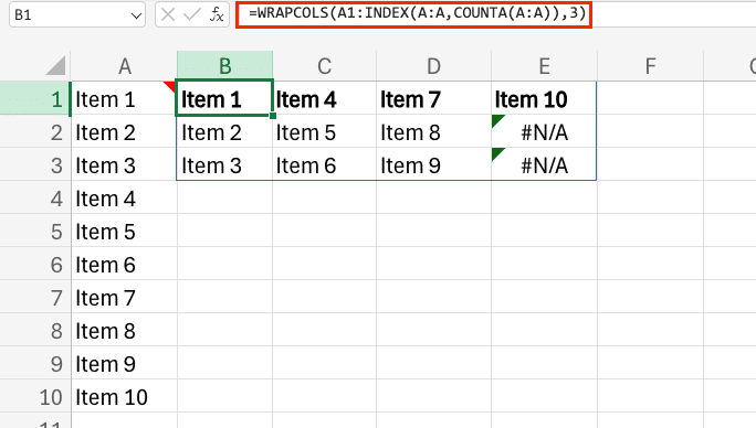
Pro tip: Combine with COUNTA to handle varying data lengths:
Copy
=WRAPCOLS(A1:INDEX(A:A,COUNTA(A:A)),3)
What is the WRAPCOLS Function?
WRAPCOLS redistributes data from top-to-bottom to left-to-right orientation. Think of it as creating a newspaper-style column layout from a single list.
Essential WRAPCOLS Parameters
Master these parameters for better control:
|
Parameter |
Purpose |
Example |
|---|---|---|
|
Vector |
Input data |
A1:A10 |
|
Wrap_count |
Column number |
3 |
|
Pad_with |
Fill empty cells |
“” or 0 |
Making the Most of WRAPCOLS
Start simple with basic layouts. Then experiment with different column counts and padding options. The key is finding the right balance for your specific needs.
Ready to take your spreadsheet capabilities further? Connect your Excel sheets to live data sources with Coefficient. Get started now and transform how you work with data.


