

Choose the cell where you want the VLOOKUP result to appear and type “=VLOOKUP(”
Enter the lookup value, the table array, and the column number index
Add “)” at the end to close the VLOOKUP function
Press “Enter” to execute the formula and return the desired output
Copy the formula to additional rows by clicking the cell and dragging the fill handle down
Want to be an expert in data extraction using Excel? VLOOKUP is the best functionality for getting targeted information from large databases. In this article, we will walk you through the basics of VLOOKUP and provide you with easy-to-use instructions on how to get the most out of this powerful tool.
Get ready to apply your data analysis tasks in the simplest way possible.
What does VLOOKUP Mean?
VLOOKUP (Vertical Lookup) is a function widely used in spreadsheet applications such as Microsoft Excel and Google Sheets. It allows users to quickly access specific data from a spreadsheet. VLOOKUP searches for a value in a specified column of a table or range and returns the corresponding value. This function offers a shortcut for extracting information from datasets without the need for manual searches. Users commonly employ VLOOKUP in inventory management, sales data analysis, and information organization to enhance efficiency and save time.
VLOOKUP Formula
The VLOOKUP formula follows a specific syntax
=VLOOKUP(lookup_value, table_array, col_index_num, [range_lookup])
The formula consists of several components that work together to perform the desired lookup. Let’s understand each component in detail:
- Lookup_value – This is the value that you need to be looking for in the first column of your table array. It works as the reference key that the VLOOKUP function uses to search for the corresponding data.
- Table_array – The table array means the row of cells which contains the data. It includes both the lookup column and columns that contain the data you will be fetching. As an example, if you look up the employee data, the table array will consist of the entire data about the employees containing the columns with the names, departments, and salaries.
- Col_index_num (Column index number) – The index of the column that will return as a result of the query is defined by this. For example, if to get the salary of an employee, the salary column is the third column in your table array, the column index number would be 3.
- Range_lookup (Range lookup (optional)) – This option allows for either an exact match or a matching value that is close. If set to TRUE or left blank, VLOOKUP will find an approximate match. If set to FALSE, it will limit the search results to exact matches. This is an attribute commonly used when handling numerical data or when sorting lists.
Example Formula:
=VLOOKUP(A2, B2:E10, 3, FALSE)
In this formula:
1. A2 is the cell containing the product ID we want to search for.
2. B2:E10 is the range of cells containing the product IDs and prices.
3. 3 indicates that we want to retrieve the data from the third column (price column).
4. FALSE specifies that we want an exact match for the product ID.
Preparing Data for VLOOKUP
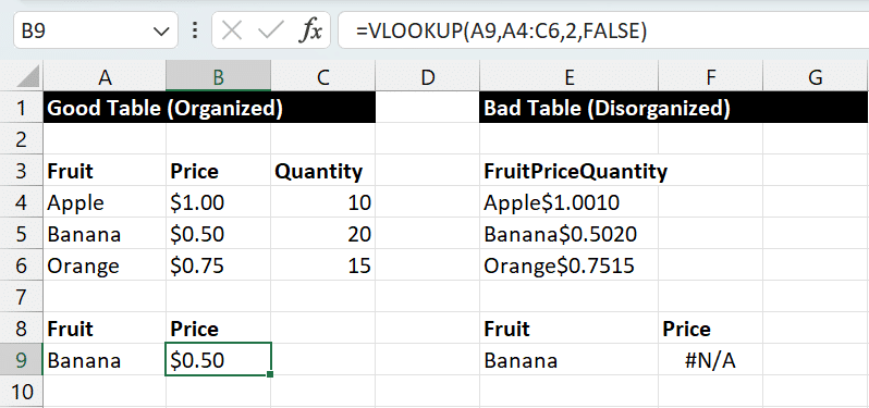
Before starting the VLOOKUP function, it is essential to prepare data correctly and it is important to generate accurate results. A properly done table is a sign of efficiency, whereas one with an incorrect structure can cause errors.
In the good table, each data category occupies its own column, facilitating VLOOKUP usage. Conversely, the bad table combines data making it challenging to identify specific values.
Below is an example illustrating the difference:
Video Tutorial
Check out the tutorial below for a complete video walkthrough!
How to use VLOOKUP in Excel
Step 1: Select the Cell for VLOOKUP
Choose the cell where the outcome of the VLOOKUP function will be displayed. This is the starting point for executing the VLOOKUP function. Ensure that the chosen cell is where the extracted data will be placed.
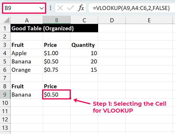
In this example, cell B9 displays the VLOOKUP value because you applied the function to this cell.
Step 2: Enter the VLOOKUP Formula
Begin by selecting the cell where you want to insert the function and type “=VLOOKUP(” into it. Next, enter the lookup value, highlight the table array to define the data range, select the column number, and choose the range lookup option if needed. Finally, add the closing parenthesis “).” For clarity, here’s an example:
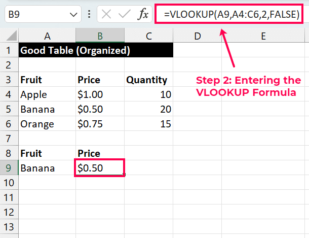
In this example, we’re searching for the value in cell B9 within the range A4:C6, searching the second column, and confirming the correctness of the result.
Step 3: Add the Lookup Value
To make the best use of the VLOOKUP function, you need to type in the precise value you want to find in your dataset. This refers to a starting point where we initiate the search process.
For example, if you need to get some information about a specific product in a sales dataset, then you should enter the product name or ID. Below is a live example demonstrating the process:
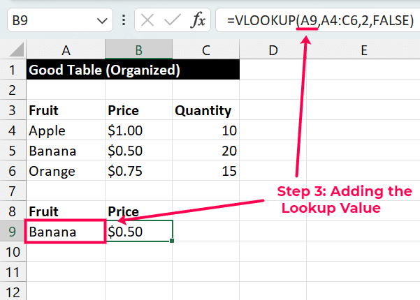
In the given example, if you enter “A9” as the lookup value, VLOOKUP will search for the corresponding Fruit “Banana”.

Stop exporting data manually. Sync data from your business systems into Google Sheets or Excel with Coefficient and set it on a refresh schedule.
Get Started
Step 4: Select the Table Array
In this step, highlight the range of cells containing the data to search in. This ensures accuracy in lookup. For example, if searching for price, select the entire price list.
Ensure the selected range includes the lookup value’s corresponding data column. Below illustrates this:
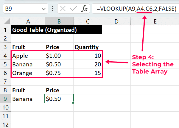
For instance, to search for the price of the Fruit “Banana”, select the range A4:C6. This action optimizes VLOOKUP’s efficiency and accuracy.
Step 5: Specify the Column Index Number
Specify the column index number to retrieve desired data. Identify the column containing the data you need in the table array. Ensure accuracy, as incorrect index numbers lead to inaccurate results. For example, if you are looking for prices, and prices are in the second column, the column index number would be 2. Below is a live example:
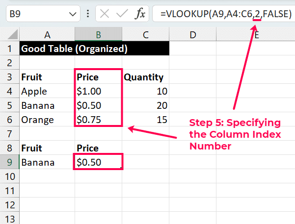
In this example, if searching for the price of bananas, the column index number would be 2.
Step 6: Choose the Range Lookup Option (if applicable)
Decide whether you want an exact match or an approximate match. When using VLOOKUP, it’s crucial to determine if you need an exact match or an approximate match based on your data and requirements.
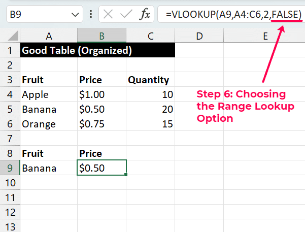
In this, we used FALSE for an exact match. If we were to use TRUE or omit the parameter, VLOOKUP would look for an approximate match, which might not yield accurate results.
Step 7: Close the Formula and Press Enter
After specifying the column index number, ensure the formula is complete by adding “)” at the end. This shows the closure of the VLOOKUP function. Pressing “Enter” is the key step towards running the VLOOKUP formula. Unlike many other Excel functions, VLOOKUP doesn’t require pressing a specific key combination (like Ctrl+Enter) to confirm the formula.
Simply pressing ‘Enter’ tells Excel to execute the formula and return the desired output. Enter the lookup value, the table array, and the column number index, and then press the Enter key to get your desired outcome.
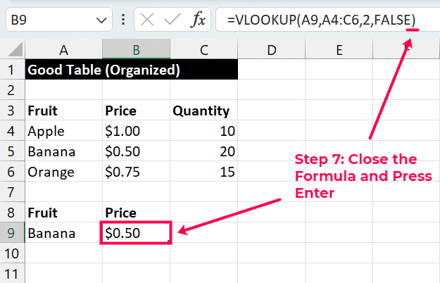
In our example, the formula “=VLOOKUP(A9,A4:C6,2,FALSE)” is used for searching the price of a banana. Hitting Enter instructs Excel to get the price of Banana from the table array given.
Simplify Business Operations with VLOOKUP
VLOOKUP proves useful across various business cases. Here are some examples:
- HR – One example is that it makes it easy to search for employee names from a large database without any effort, hence the HR processes are simplified.
- Inventory – Just as the process of pulling up product prices from lengthy price lists gets easy, inventory management and price strategies are also made more efficient.
- Sales – VLOOKUP is a very useful tool in sales and customer service. It can quickly search for important customer information from databases, making the interaction with clients to be more effective and the service delivery faster.
These examples, therefore, depict the flexibility and applicability of VLOOKUP in solving complicated tasks in various fields, which is the key to the efficiency and effectiveness of the decision-making processes.
Pro-tip: You can accelerate your data workflows and utilize Coefficient’s Formula Builder to automatically generate VLOOKUP formulas in Google Sheets, completing your process in just a few clicks.
Troubleshooting Common Issues
While the VLOOKUP function in Excel is a useful tool, mistakes in its usage are not uncommon. Here are the key points to address common issues:
- #N/A error – It occurs when the lookup value is absent from the dataset. A typo or a non-existent value in the lookup column frequently causes this issue.
- Incorrect results – If the array that holds the table is defined wrongly or the column index number is incorrectly specified, the program may produce incorrect results. It is advisable to cross-check the values of these factors to overcome this problem.
- Data not sorted – In the absence of the sorting feature and the approximate match technique, one cannot neglect the possibility of inaccuracy in the results. It is important to ensure that the data is sorted in ascending order for VLOOKUP to work correctly when there is an approximate match.
VLOOKUP Function: Tips and Best Practices
Being proficient in the application of the VLOOKUP function in Excel will greatly expand data extraction and analysis capabilities. To make the most of this powerful tool, consider the following tips, best practices, and important reminders:
- Dynamic Column Index – Make your VLOOKUP formulas more adaptable by applying the MATCH function to dynamically adjust the column index. This is very important when working with tables that often have structural changes.
- Wildcard Usage – Apply wildcard characters to stand for any character and any single character respectively to expand search criteria when exact matches are not necessary, and consequently, the flexible nature of your search process will be enhanced.
- Case Sensitivity – Keep in mind that VLOOKUP is case-insensitive that is it is not affected by the letter case in any way.
- Error Handling – Being ready to answer questions like #N/A!, #REF!, #VALUE!, and #NAME! is a must for you. through the use of the correct error-handling techniques and by maintaining uniform data formats.
- Quoting Lookup Values – Make sure you put lookup values in quotes or use correct cell references so that #NAME! doesn’t appear. detect and correct errors as well as guarantee correct data acquisition.
- Best Practice for Lookup Values – While using text as lookup values, make sure that they are enclosed in quotes or refer to cells instead of using text so that there will not be any errors and the formulas will be consistent.
Unlock Excel’s Power with Coefficient
With the addition of skills like VLOOKUP and the use of Coefficient, your skills in Excel data management can be greatly improved.
Coefficient takes the headache out of keeping your spreadsheets up-to-date by automatically handling the data import and refresh process. Together with Coefficient, you simplify workflows, eliminate manual tasks, and ensure your data is always up to date, thus making decisions based on data instead of conjectures.
Discover the opportunities with Coefficient and boost your Excel skills to improve your performance.


