Use the “&” operator to combine multiple criteria into a single lookup value
Create a lookup value that concatenates your search criteria using the “&” operator
Adjust the lookup array to match your combined criteria by concatenating the corresponding columns in the same format
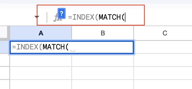
Build the formula starting with =INDEX(return_range, then add MATCH(lookup_value1&lookup_value2, and concatenate your lookup values
Use array formulas by pressing Ctrl+Shift+Enter (Windows) or Cmd+Shift+Enter (Mac) to handle multiple criteria
Want to perform complex lookups in Google Sheets? Learn to combine INDEX and MATCH functions for multi-criteria searches, enhancing your data analysis capabilities.
Setting Up INDEX and MATCH for Multiple Criteria Lookup
Creating the Basic Formula Structure
To use INDEX and MATCH with multiple criteria, we need to construct a formula that combines these functions effectively. Let’s break it down step-by-step.
Step 1. Start with the INDEX function as the outer function.
- Begin your formula with =INDEX(

- This function will return the value we’re looking for once we’ve found its position.
Step 2. Nest the MATCH function inside INDEX for row lookup.
- Inside the INDEX function, add MATCH(

- MATCH will find the position of our lookup criteria within a specified range.
Step 3. Use array formulas to handle multiple criteria.
- To work with multiple criteria, we’ll need to use array formulas.
- After completing your formula, press Ctrl+Shift+Enter (Windows) or Cmd+Shift+Enter (Mac) to create an array formula.
Incorporating Multiple Criteria into MATCH
To search using multiple criteria, we need to combine our search terms and adjust our lookup array accordingly.
Step 1. Use the “&” operator to combine multiple criteria.
- The “&” operator allows you to concatenate text strings.
- Use it to join your search criteria into a single lookup value.
Step 2. Create a lookup value that concatenates your search criteria.
- Combine your search terms using the “&” operator.
- For example: =MATCH(A2&B2, C2:C100&D2:D100, 0)

Step 3. Adjust the lookup array to match your combined criteria.
- Modify your lookup array to concatenate the corresponding columns.
- This ensures your lookup value and array use the same format.
Implementing INDEX and MATCH with Two Criteria
Step-by-Step Formula Construction
Let’s construct a formula that uses INDEX and MATCH with two criteria.
Step 1. Begin with =INDEX(return_range,
- Start your formula by specifying the range containing the values you want to return.
- For example: =INDEX(E2:E100,

Step 2. Add MATCH(lookup_value1&lookup_value2,
- Inside the INDEX function, start the MATCH function.
- Concatenate your two lookup values.
- Example: =INDEX(E2:E100,MATCH(A2&B2,

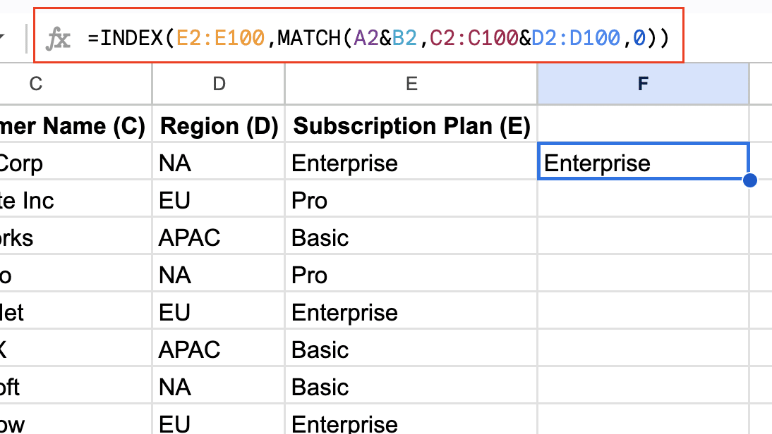
Step 3. Complete with lookup_array1&lookup_array2,0))
- Finish the MATCH function by specifying your lookup array and match type.
- Example: =INDEX(E2:E100,MATCH(A2&B2,C2:C100&D2:D100,0))

Step 4. Press Ctrl+Shift+Enter to create an array formula.
- After entering your formula, use the array formula shortcut.
- This tells Google Sheets to treat the formula as an array formula.
Handling Different Data Types in Criteria
When working with multiple criteria, you may encounter different data types. Here’s how to handle them:
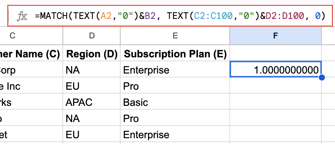
Step 1. Convert numbers to text using the TEXT function if necessary.
- If one of your criteria is a number, use TEXT to convert it to a string.
- Example: =MATCH(TEXT(A2,”0″)&B2, TEXT(C2:C100,”0″)&D2:D100, 0)

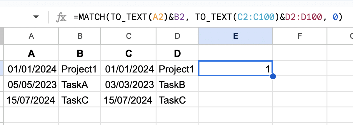
Step 2. Use the TO_TEXT function for dates in your criteria.
- For date criteria, use TO_TEXT to ensure consistent formatting.
- Example: =MATCH(TO_TEXT(A2)&B2, TO_TEXT(C2:C100)&D2:D100, 0)

Step 3. Ensure consistent formatting across your lookup values and arrays.
- Make sure the format of your lookup value matches the format in your lookup array.
- This may involve using functions like TEXT or TO_TEXT on both sides of the MATCH function.
Expanding to Three or More Criteria
Modifying the Formula for Additional Criteria
Adding more criteria to your INDEX and MATCH formula is straightforward. Here’s how to do it:
Step 1. Add more lookup values to the MATCH function.
- Include additional criteria in your MATCH function, separated by “&”.
- Example: =INDEX(F2:F100,MATCH(A2&B2&C2,
Step 2. Expand the lookup array to include all criteria columns.
- Add corresponding columns to your lookup array, also separated by “&”.
- Example: =INDEX(F2:F100,MATCH(A2&B2&C2,D2:D100&E2:E100&F2:F100,0))

Step 3. Adjust the formula structure to accommodate the new criteria.

Stop exporting data manually. Sync data from your business systems into Google Sheets or Excel with Coefficient and set it on a refresh schedule.
Get Started
- Ensure your INDEX range reflects the correct column for returned values.
- Double-check that all criteria and array ranges are correctly aligned.
Managing Complex Data Sets
When dealing with large or complex datasets, consider these strategies:
Step 1. Use helper columns to simplify your lookup process if needed.
- Create additional columns that combine multiple criteria.
- This can make your main formula simpler and easier to manage.
Step 2. Consider using FILTER function alongside INDEX-MATCH for large datasets.
- For very large datasets, FILTER can be more efficient.
- Example: =INDEX(FILTER(F2:F100,(D2:D100=A2)*(E2:E100=B2)*(F2:F100=C2)), 1)

Step 3. Optimize formula performance by limiting the lookup range.
- Restrict your lookup range to only the necessary data.
- This can significantly improve calculation speed for large spreadsheets.
Returning Multiple Values with INDEX and MATCH
Creating an Array of Results
Sometimes, you may want to return multiple values that match your criteria. Here’s how:
Step 1. Modify the INDEX function to return a range instead of a single cell.
- Change your INDEX range to include multiple columns.
- Example: =INDEX(E2:G100, MATCH(A2&B2, C2:C100&D2:D100, 0), {1,2,3})

Step 2. Use the TRANSPOSE function to display results horizontally if needed.
- Wrap your formula in TRANSPOSE to change the orientation of results.
- Example: =TRANSPOSE(INDEX(E2:G100, MATCH(A2&B2, C2:C100&D2:D100, 0), {1,2,3}))

Step 3. Implement error handling to manage cases with no matches.
- Use IFERROR to provide a custom message when no match is found.
- Example: =IFERROR(INDEX(E2:G100, MATCH(A2&B2, C2:C100&D2:D100, 0), {1,2,3}), “No match found”)

Combining with Other Functions for Advanced Analysis
Enhance your data analysis by combining INDEX and MATCH with other functions:
Step 1. Integrate SUMIFS or COUNTIFS for numerical analysis of matched data.
- Use these functions to perform calculations on your matched results.
- Example: =SUMIFS(E2:E100, C2:C100, A2, D2:D100, B2)
Step 2. Use VLOOKUP in combination with INDEX-MATCH for more flexible lookups.
- Combine these functions for complex, multi-step lookups.
- Example: =VLOOKUP(INDEX(E2:E100, MATCH(A2&B2, C2:C100&D2:D100, 0)), F2:G100, 2, FALSE)

Step 3. Explore QUERY function for complex data manipulation tasks.
- For advanced data analysis, consider using the QUERY function.
- Example: =QUERY(B2:E100, “SELECT E WHERE C = ‘”&A2&”‘ AND D = ‘”&B2&”‘”)

Understanding the Power of INDEX and MATCH
Advantages Over VLOOKUP
INDEX and MATCH offer several benefits compared to VLOOKUP:
- Flexibility in column order: Unlike VLOOKUP, INDEX and MATCH don’t require your lookup column to be the leftmost in your range.
- Ability to perform right-to-left lookups: INDEX and MATCH can search in any direction, not just left-to-right like VLOOKUP.
- Enhanced performance with large datasets: For extensive data ranges, INDEX and MATCH often calculate faster than VLOOKUP.
How INDEX and MATCH Work Together
Understanding the individual roles of INDEX and MATCH helps in utilizing their combined power:
- INDEX: Returns a value from a specified position in a range. It answers the question, “What value is in this specific row and column?”
- MATCH: Finds the position of a lookup value within an array. It tells you, “Where in this range is my lookup value?”
- Combining them allows for dynamic, criteria-based lookups. MATCH finds the position, which INDEX then uses to return the corresponding value.
By mastering INDEX and MATCH with multiple criteria, you’ve expanded your data lookup capabilities in Google Sheets. Apply these techniques to enhance your spreadsheet analysis.
Ready to take your Google Sheets skills to the next level? Try Coefficient to seamlessly sync live data from your business systems directly into your spreadsheets. Get started with Coefficient and transform your data workflow today.

