Introduction To SUMIFS Excel Function
The SUMIFS function in Excel can help you get the sum of a range of cells that meet specific conditions. However, you can use it with a single criteria (where it functions identically to the SUMIF function), or you can use it with multiple criteria.
It can be a little challenging to figure out exactly how to use the SUMIFS function to return the result you want. But we’re going to clear away all that confusion in this article and show you some practical examples of using SUMIFS.
So let’s get started with the syntax and parameters first.
SUMIFS Excel Function Syntax And Parameters
The basic syntax for the SUMIFS function is as follows:
=SUMIFS(sum_range, criteria_range1, criteria1, [criteria_range2, criteria2], …)
This structure allows you to specify the range you want to sum and the criteria you want to apply to one or more other ranges. The result is a calculated sum considering all the conditions you’ve set.
Let’s look at each of the parameters in detail:
- The “sum_range” parameter specifies the range cells that contain the values to be summed.
- The “criteria_range1” parameter specifies the range of cells that will be evaluated against the first criteria. This criteria range must be the same size and shape as the sum_range.
- The “criteria1” parameter is the condition or value that will be used to filter the data in “criteria_range1”. This can be a number, text, or logical expression.
- The optional parameters “criteria_range2” and “criteria2” allow additional criteria to be applied. These work as the “criteria_range1” and “criteria1” parameters.
- You may also use additional criteria range and parameters up to a maximum of 29.
The SUMIFS function can help you perform complex calculations and extract meaningful insights from your data by carefully selecting the appropriate sum_range, criteria ranges, and criteria values.
SUMIF vs. SUMIFS: Differences
We mentioned earlier that the SUMIF function is similar to the SUMIFS function. Let’s look at the syntax to see how they’re different.
The syntax of SUMIF is: =SUMIF(range, criteria, [sum_range])
Where:
- range defines the range of cells to be evaluated.
- criteria is the condition that will be used to filter the values for summing.
- sum_range is an optional argument you can use if the cells to sum are different from array.
As you can see from the syntax, SUMIF takes only one criteria in its arguments. Thus, making the SUMIFS function the more versatile of the two.
NOTE: The criteria range arguments must have the same dimension as the summed range. This means that the number of columns in the criteria ranges must match the number of columns in the range being summed for the SUMIFS function to work correctly. This is because the SUMIFS function compares each row in the criteria ranges to the corresponding row in the range being summed and only includes the values in the sum if all the criteria are met.
Don’t worry if this is your first time using the SUMIFS function. An example will help clarify things.
Video Tutorial
Check out the tutorial below for a complete video walkthrough!
Practical Examples Of The Excel SUMIFS Function
Let’s say you’re a mobile phone manufacturer who makes three kinds of phones:
- Basic Phone
- Smartphone
- Foldable Smartphone
And you sell your product in the following three countries:
- USA
- UK
- Germany
Here’s what your sales data might look like:
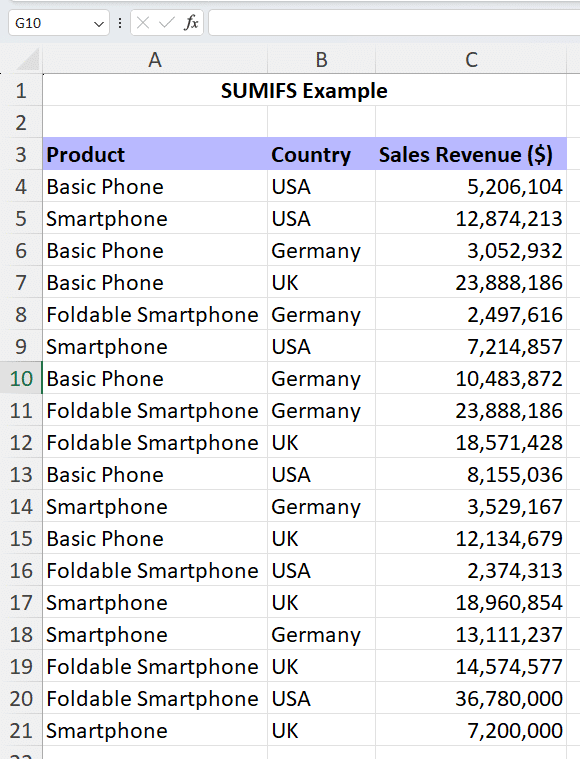
Let’s examine a few examples of summing the total revenue based on different criteria.
Example #1: Using SUMIFS For Single Criteria
You could use the SUMIF function to calculate the total sales revenue of all the “Basic Phones” sold across all countries. But in this example, we’ll demonstrate how the SUMIFS function can replace it.
Step 1: Start writing the SUMIFS function in the cell where you desire to see the total sales revenue. In this case, H4.
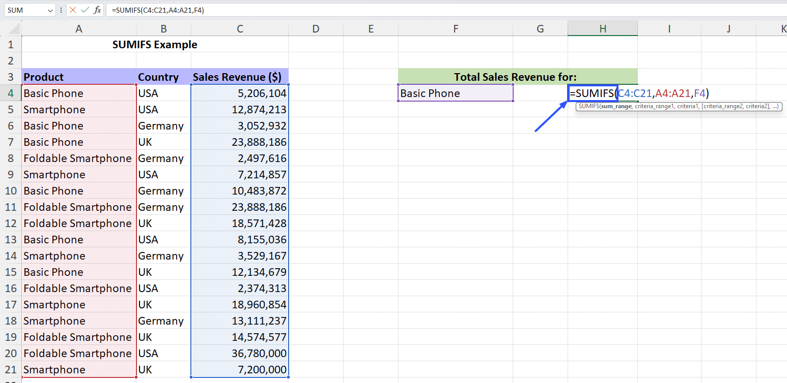
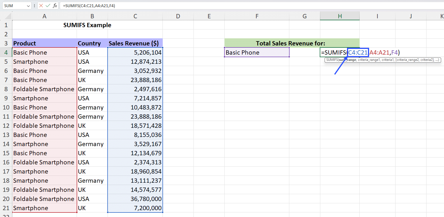
Step 2: As the first parameter, input the range from which you want the sum calculated. In this case, the sales revenue figures.
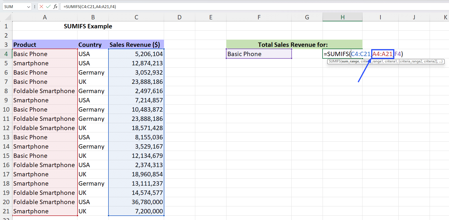
Step 3: The second parameter calls for selecting the range in which the criteria will be matched with each entry. In this case, the Product column.
Step 4: The following parameter is the criteria itself (“Basic Phone”). For ease of reference, we’ve copied this criteria to cell F4.
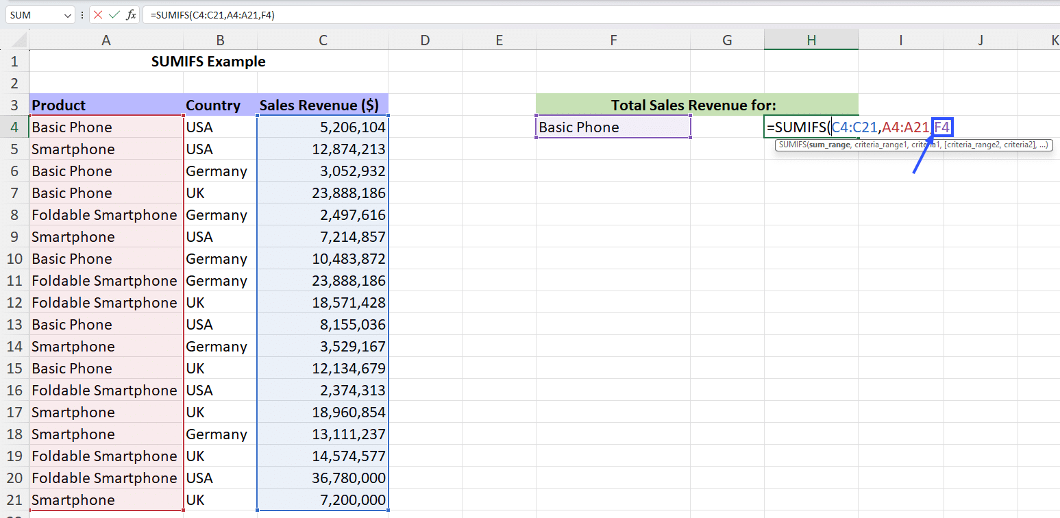
Step 5: End the SUMIFS formula with the right parentheses and hit enter to calculate the sum.
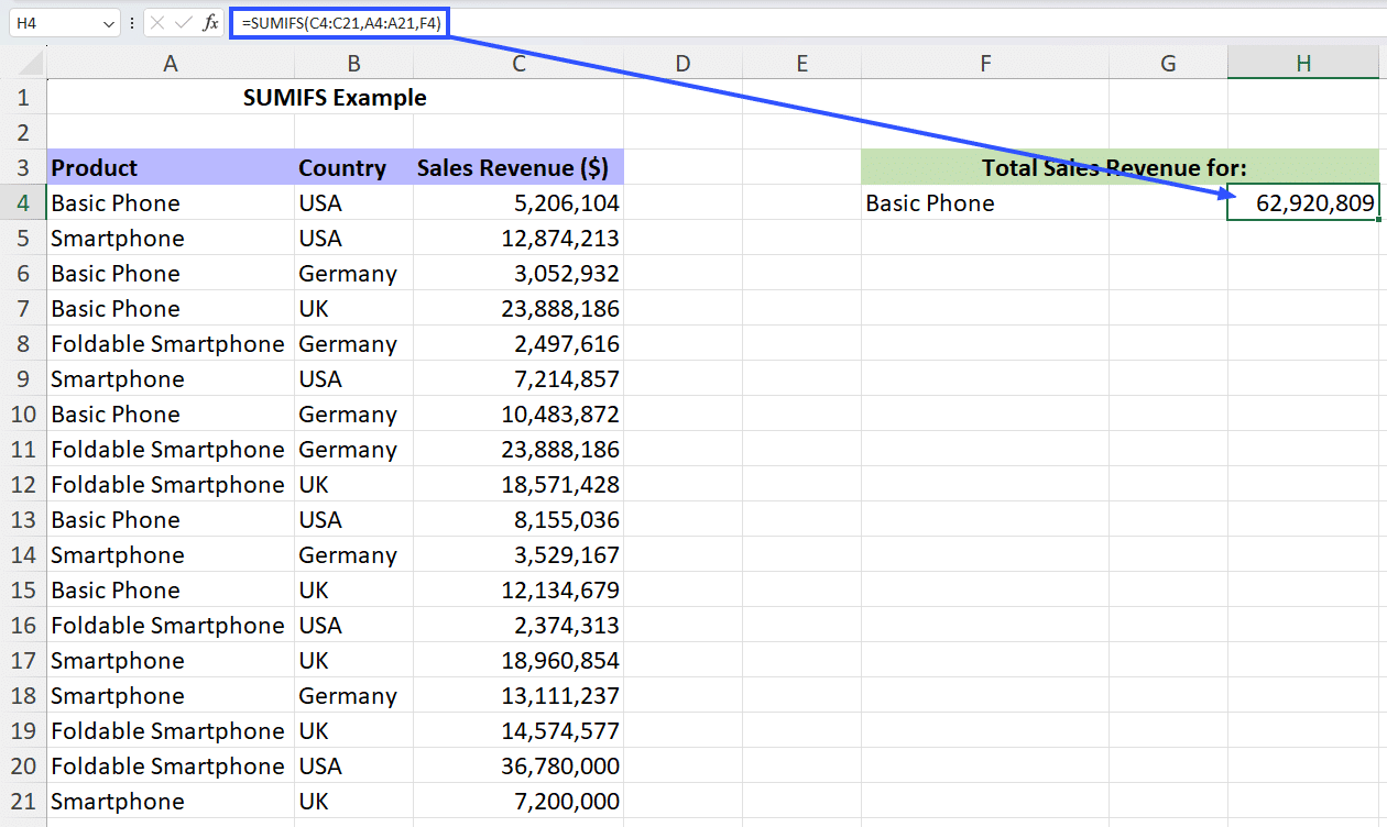
Step 6: You can verify the total by manually tallying the sales revenue figure against each “Basic Phone” entry.
The formula we used to calculate the total with a single parameter is: =SUMIFS(C4:C21,A4:A21,F4)
Next, let’s see how to calculate the total using multiple criteria.
Example #2: Using SumIFS For Multiple Criteria
Let’s calculate the total sales revenue of all the “Foldable Smartphones” sold in the “UK,” we’ll use the SUMIFS function with two parameters.
Step 1: We’ll follow steps 1-4 from the previous example but with the following parameters:
- sum_range is the same as the previous example, C4:C21.
- criteria_range1 is the same as the previous example, A4:A21, since we’ll evaluate the criteria in the same range of entries.
- The first criteria for this case is “Foldable Smartphones,” which we’ve copied to cell F5. So, the criteria1 parameter is F5.
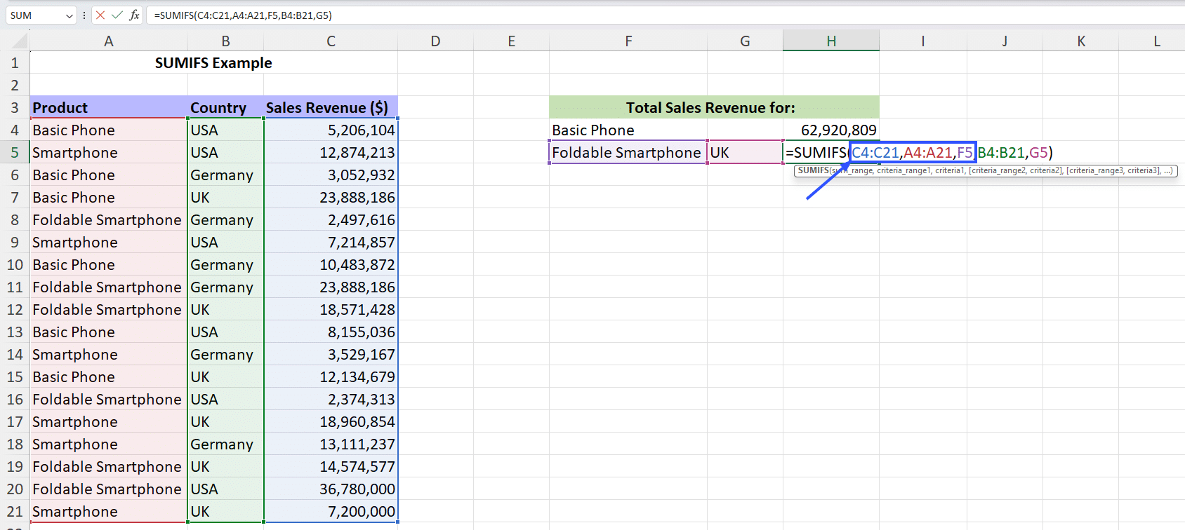
Step 2: Next, we enter the parameters for the second criteria, i.e., “UK.” For this criteria, the parameters are:
- criteria_range2 is all the entries in Column B, B4:B21.
- The criteria is “UK,” which we’ve copied to cell G5 for reference. So, the criteria2 parameter is G5.
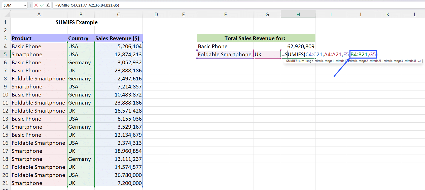
Step 3: End the SUMIFS formula with the right parentheses and hit enter to calculate the sum. You can manually tally the total to verify the result.
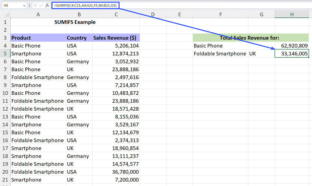
The formula we used to calculate the total with a single parameter is: =SUMIFS(C4:C21,A4:A21,F5,B4:B21,G5)
You can follow the same steps to calculate the sum from your data using even three or more variables.
But wait. The SUMIFS function offers even more functionality, which is what makes it so versatile and powerful for data analytics. Let’s take a look.
Example #3: Using Comparison Operators
When using the SUMIFS function in Excel, you can also use comparison operators (‘=’, ‘>’, ‘<’, ‘<=’, ‘>=’, ‘<>’) as part of the determining criteria for the sum calculation.
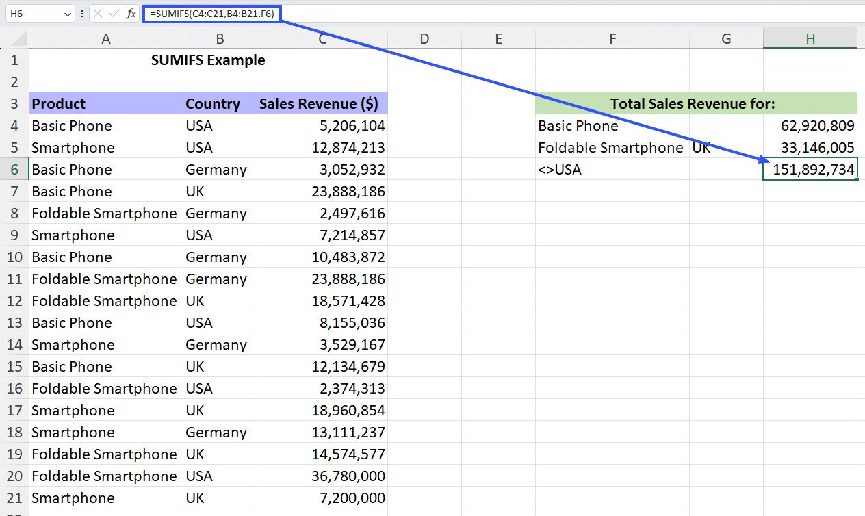
Let’s say you want to calculate the total sales revenue for all the products across all countries except the USA, you can use the not equal to operator ‘<>’ in the criteria. So the criteria range will be all the values in Column B, and the criteria will be “<>USA”.
In this example, you’d use the formula as follows: =SUMIFS(C4:C21,B4:B21,F6)
Example #4: Use Of Wildcards For Dynamic Criteria
Wildcards characters, such as the asterisk (‘*’), question mark (‘?’), and blank space (‘ ‘), can be used to create dynamic and flexible criteria when using the SUMIFS Excel function.
If you want to calculate the total sales revenue for all the smartphones, you’d need to include “Smartphones” and “Foldable Smartphones” in the criteria. You may think using “<>Basic Phone” would also work. And you’re right! It’ll give you the result you want.
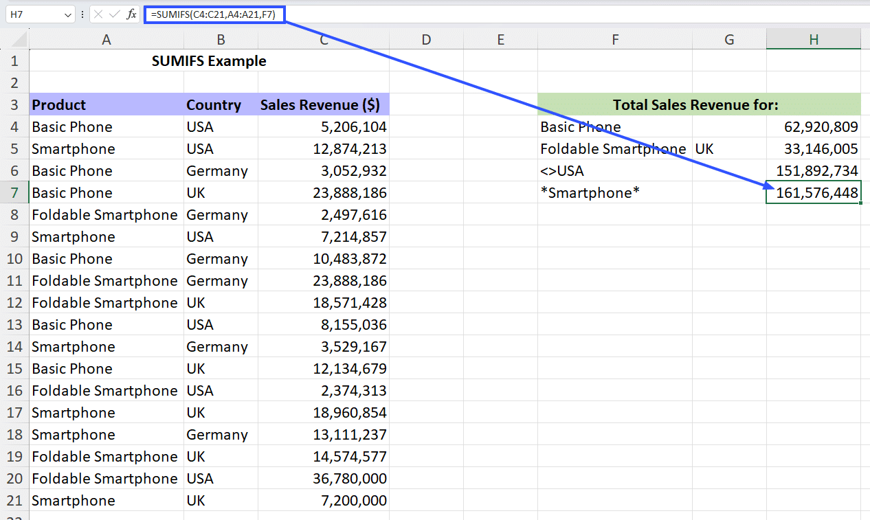
However, if there were a dozen different products and only some were smartphones, the “<>” criteria wouldn’t cut it. You can use the asterisk (‘*’) wildcard to check for product names with the word “Smartphone” in it.
So the criteria range will be all the values in Column A, and the criteria will be “*Smartphone*”.
In this example, you’d use the formula as follows: =SUMIFS(C4:C21,A4:A21,F7)
Remember, you can use a single or multiple criteria to do a conditional summation operation on your data set using the SUMIFS function in Excel. Wildcards and comparison operators only add another level of granularity and flexibility.
Next, let’s look at some advanced uses of the SUMIFS Excel function.
Advanced Uses Of The SUMIFS Excel Function
Here are some ways to use SUMIFS that goes beyond its basic application:
Handling Blank And Non-Blank Cells
If your data set contains blank values, you can use the argument “=” to specify using blank cells for the criteria. Similarly, you can use the argument “<>” to specify using non-blank cells for the criteria.
Let’s look at an example of each.
If you use the formula: =SUMIFS(D4:D21,C4:C21,”=”)
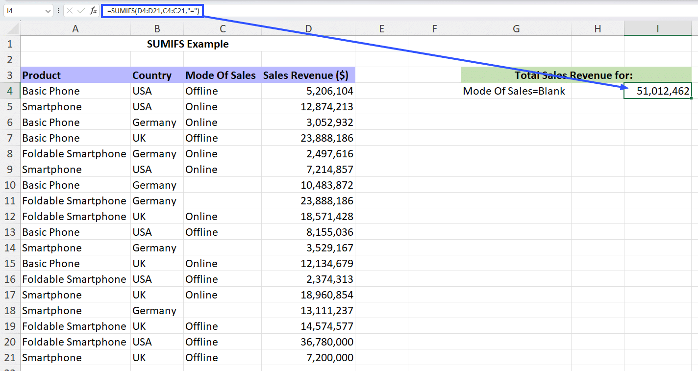
The function will return the sum of all values in the Sales Revenue column that meet the criteria Mode Of Sales is blank.

Stop exporting data manually. Sync data from your business systems into Google Sheets or Excel with Coefficient and set it on a refresh schedule.
Get Started
But if you use the formula: =SUMIFS(D4:D21,C4:C21,”<>”)
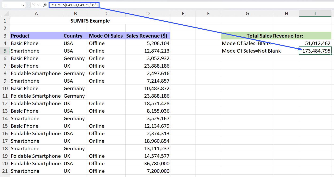
The function will return the sum of all values in the Sales Revenue column that meet the criteria Mode Of Sales is not blank.
Summing Values Based On Dates Using TODAY Function
You can calculate the sum of a range of cells based on a date criteria that you specify, since Excel treats dates as numbers. However, you can also use the TODAY function within the formula to do this calculation.
So you’ll write the formula as: =SUMIFS(D4:D21,C4:C21,”>=”&TODAY())
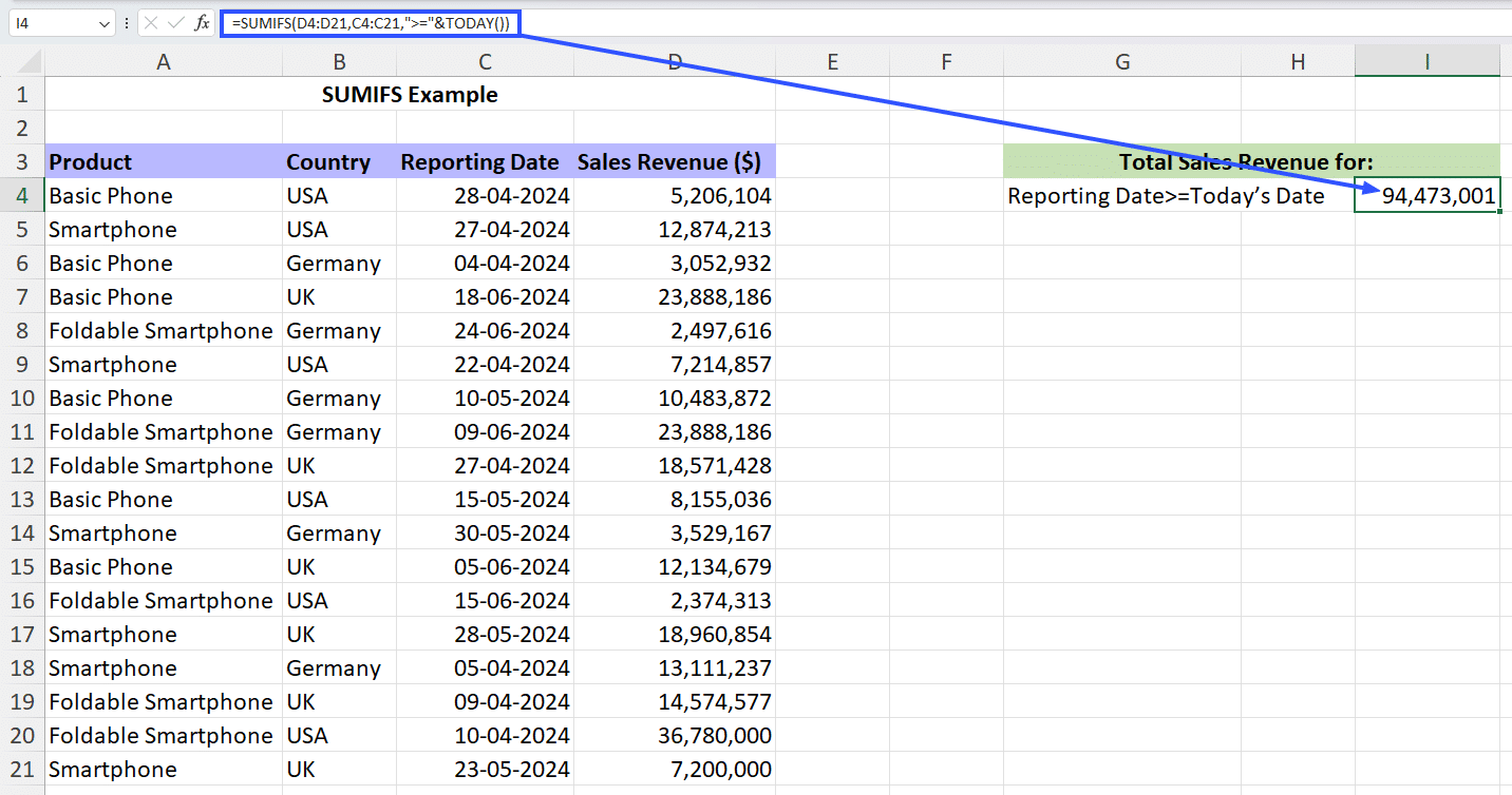
This function will return the sum of all the cells in the Sales Revenue column if they match the criteria Reporting Date>=Today’s Date.
Summing Sales Data Based on Multiple Conditions
Scenario: You have a sheet in which you have added sales data and want to sum the amount of sales for a precise product classification in a specific region during a precise quarter.

Aim: Sum the amount of sales for the “Electronics” classification in the “North” region during “Q1”.
Formula: =SUMIFS(E2:E9, B2:B9, “Electronics”, C2:C9, “North”, D2:D9, “Q1”)

Outcome: 2400
Summing Employee Hours Based on Multiple Criteria
Scenario: You have a timesheet of employees and want to sum the total hours operated by employees in a precise department who operated more than a definite number of hours in a given week.

Aim: Sum the hours of working by employees in the “HR” department who operated more than 40 hours in week 1.
Formula: =SUMIFS(D2:D9, B2:B9, “IT”, C2:C9, 1, D2:D9, “>40”)

Outcome: 44
We’re sure you’ll find these uses of SUMIFS quite handy, but that’s not all you can do with this function. Let’s look at some more advanced uses.
Methods For Using SUMIFS with Multiple OR Criteria
The SUMIFS function criteria takes an AND logic approach, but if you want to run a summing operation on a data set with multiple OR criteria, here’s what you could do:
#1 Combining SUMIFS Excel Functions For OR Logic Scenarios
If you have multiple OR criteria for a summing operation, you could simply sum up multiple SUMIFS Excel functions, each with its own criteria.
The formula for that would look like this: =SUMIFS(D4:D21,B4:B21,G4,A4:A21,H4)+SUMIFS(D4:D21,B4:B21,G5,A4:A21,H5)+SUMIFS(D4:D21,B4:B21,G6,A4:A21,H6)
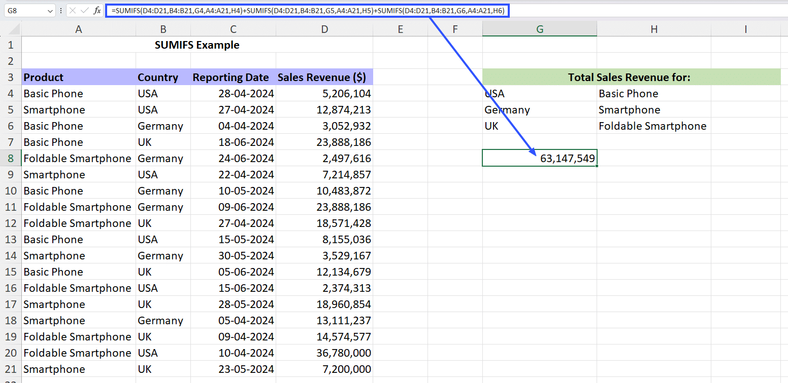
Despite looking like a very long, cumbersome formula, this simply returns the sum of all the sales revenue figures in column D, as long as it meets the criteria {Country: USA AND Product: Basic Phone} OR {Country: Germany AND Product: Smartphone} OR {Country: UK AND Product: Foldable Smartphone}.
#2 Using Array Arguments With SUM And SUMIFS Excel Function
Another way is to define the different OR criteria as an array in the SUMIFS argument, which would return the sum of each OR criteria in a separate cell. Then, if you encapsulate the SUMIFS function in SUM, it should give you the desired result.
This what the formula looks like: =SUM(SUMIFS(D4:D21,B4:B21,{“USA”,”UK”}))
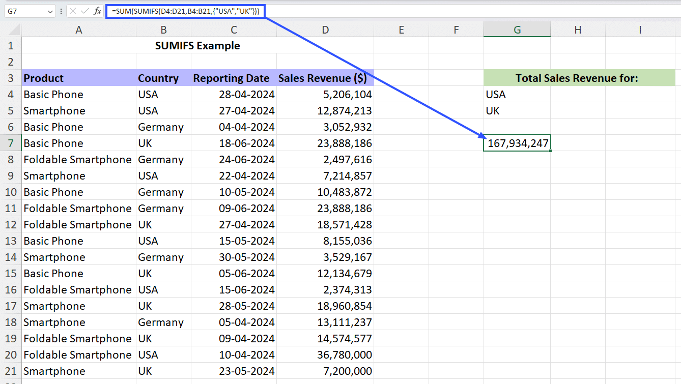
This function returns the sum of all the sales revenue figures in column D if the country is USA or UK.
As you can see, the more criteria you use, the more convoluted the SUMIFS Excel function becomes. To mitigate this issue, you can use Named Ranges.
Enhancing SUMIFS With Named Ranges In Excel
By leveraging Named Ranges, you can create more intuitive and self-documenting formulas that are easier to understand and maintain. Named Ranges allow you to clearly define the criteria ranges, making it simpler to reference and modify the relevant data sources when using the SUMIFS Excel function.
Using Named Ranges not only enhances the formula’s clarity but also reduces the risk of errors that can occur when manually referencing cell ranges. It also helps you update the source data without the need to adjust the formula itself, thus making your spreadsheets more adaptable and responsive to changes.
Practical Tips For Efficient SUMIFS Formulas
Here are some practical tips to help you make efficient use of the SUMIFS Excel function:
- Check Syntax: Verify that the syntax of your SUMIFS function is correct and the range to sum, criteria range(s), and criteria(s) have been specified in the correct order.
- Verify Criteria Range: Ensure that the criteria range(s) in your SUMIFS function are valid and include the correct cells or range of cells. If the criteria range is incorrect, the function may return errors.
- Verify Criteria: Check that the criteria(s) you are using in the SUMIFS function match the data in the criteria range(s). Mismatched criteria can lead to incorrect results or errors.
- Check for Data Type Mismatch: Make sure that the data types of the criteria match the data types in the criteria range(s). For example, if you are comparing text values, ensure that both the criteria and criteria range contain text.
- Use Wildcards Properly: If you are using wildcards (* or ?) in your criteria, ensure that they are used correctly and do not cause unintended filtering of data.
- Handle Errors Correctly: Use error handling functions like IFERROR to display custom messages or handle errors correctly in case the SUMIFS Excel function encounters issues.
- Use Evaluate Formula Tool: Excel’s “Evaluate Formula” tool can help you step through the calculation of the SUMIFS function to identify any specific issues or errors in the formula.
- Check for Hidden Cells or Rows: Hidden cells or rows that are part of the criteria range(s) can impact the results of the SUMIFS function. Unhide any hidden cells or rows before using the function.
- Ensure Consistent Data Format: Ensure that the data format is consistent across the criteria range(s) and criteria(s) to avoid errors related to formatting discrepancies.
With these tips, chances of encountering common errors (like #NAME?, #REF!, #VALUE!, etc.) will be reduced. If they do occur, troubleshoot them as usual.
In addition, optimizing the SUMIFS Excel function for large datasets can improve the efficiency and accuracy of your data analysis. The key lies in breaking down the formula into its core components, identifying the most critical criteria, and streamlining the syntax to minimize processing time.
This approach not only ensures that your calculations are fast, but also enhances the readability and maintainability of your spreadsheets, making them easier to understand and update as your data changes.
Now, it’s time to sum up our discussion on the SUMIFS Excel function.
Using The SUMIFS Excel Function
We hope this guide has demonstrated how to use SUMIFS with multiple criteria in Excel to easily filter your data and calculate your desired sums.
That doesn’t take away from the endless hours spent manually pushing and pulling data into Excel. Imagine having to copy live data multiple times a day and running the SUMIFS function repeatedly.
But with Coefficient, you can say goodbye to repetitive tasks and hello to efficiency. It is the leading spreadsheet automation tool which connects to any data source, imports live data, and automates spreadsheet workflows. Get started with Coefficient today.
