Excel ROUND Function Tutorial: Master Precise Data Rounding (2024)

Excel’s ROUND function truncates decimals to specified places. It’s crucial for financial calculations, data analysis, and reporting accuracy.

Tutorial: Using the ROUND Function in Excel

The ROUND function in Excel is designed to round numbers to a specified number of digits. Its basic syntax is:

=ROUND(number, num_digits)

Where:

• ‘number’ is the value you want to round
• ‘num_digits’ specifies how many decimal places to round to

Let’s walk through how to apply this function step-by-step:

Step 1: Open your Excel spreadsheet

• Navigate to the cell where you want the rounded result to appear.
• Click on the cell to select it.

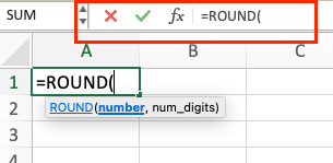
Step 2: Enter the ROUND function

• Type an equals sign (=) to start the formula.
• Type ROUND followed by an opening parenthesis.

Step 3: Input the number to be rounded

• Enter the number you want to round, or the cell reference containing the number.
• Add a comma after the number or cell reference.

Step 4: Specify the number of decimal places

• Enter the number of decimal places you want to round to.
• Close the parenthesis.

Step 5: Press Enter to complete the formula

• Your result will appear in the cell.

Here are some examples of rounding to different decimal places:

1. =ROUND(3.14159, 2) results in 3.14

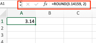
1. =ROUND(3.14159, 0) results in 3

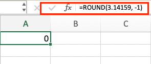
1. =ROUND(3.14159, -1) results in 0

Rounding to Specific Decimal Places

Rounding to two decimal places is common in financial calculations. Here’s how to do it:

Step 1: Select the cell for your result

• Click on the cell where you want the rounded number to appear.

Step 2: Enter the ROUND formula

• Type =ROUND(

• Enter the cell reference containing the number you want to round.
• Type ,2)
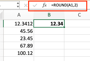
• Your formula should look like this: =ROUND(A1,2)

Step 3: Press Enter

• The result will display in your selected cell, rounded to two decimal places.

To round to the nearest whole number:

Step 1: Select your result cell

Step 2: Enter the ROUND formula

• Type =ROUND(
• Enter the cell reference with the number to round.
• Type ,0)
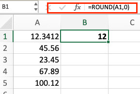
• Your formula will look like: =ROUND(A1,0)

Step 3: Press Enter

• Your result will be rounded to the nearest whole number.

For rounding to the nearest thousand:

Step 1: Choose your result cell

Step 2: Input the ROUND formula

• Type =ROUND(
• Enter the cell reference containing your number.
• Type ,-3)
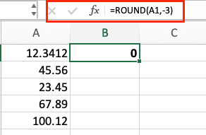
• Your formula should resemble: =ROUND(A1,-3)

Step 3: Press Enter

• The result will be rounded to the nearest thousand.

Handling Negative Numbers with ROUND

The ROUND function treats negative numbers consistently with positive ones. It rounds away from zero for midpoint values (.5 and above). For example:

• =ROUND(-3.5, 0) results in -4
• =ROUND(-3.4, 0) results in -3
• =ROUND(-3.14159, 2) results in -3.14

Here’s a step-by-step guide for rounding negative numbers:

Step 1: Select your result cell

Step 2: Enter the ROUND formula

• Type =ROUND(

• Input your negative number or cell reference.
• Add a comma and specify decimal places.
• Close the parenthesis.

Step 3: Press Enter

• Your negative number will be rounded according to the specified decimal places.

Combining ROUND with Other Excel Functions

ROUND can be integrated with other Excel functions for more complex calculations. Here’s how to use it with SUM for total calculations:

Step 1: Select your result cell

Step 2: Begin your formula

• Type =ROUND(SUM(

Step 3: Select the range to sum

• Highlight the cells you want to sum.
• Add a closing parenthesis.

Step 4: Specify decimal places

• Add a comma after the SUM function.
• Type the number of decimal places.
• Close the final parenthesis.

Step 5: Press Enter

• Your result will be the rounded sum of the selected range.

For integrating ROUND with AVERAGE:

Step 1: Choose your result cell

Step 2: Start your formula

• Type =ROUND(AVERAGE(

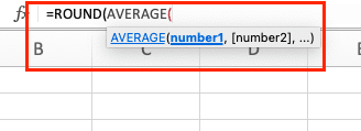
Step 3: Select the range for averaging

• Highlight the cells you want to average.
• Add a closing parenthesis.

Step 4: Specify decimal places

• Add a comma after the AVERAGE function.
• Enter the number of decimal places.
• Close the final parenthesis.

Step 5: Press Enter

• Your result will be the rounded average of the selected range.

How to Round Up a Number in Excel

The ROUNDUP function always rounds numbers up, regardless of the decimal value. Its syntax is identical to ROUND:

=ROUNDUP(number, num_digits)

Here’s how to use it:

Step 1: Select your result cell

Step 2: Enter the ROUNDUP formula

• Type =ROUNDUP(

• Enter your number or cell reference.
• Add a comma and specify decimal places.
• Close the parenthesis.

Step 3: Press Enter

• Your number will be rounded up to the specified decimal places.

ROUNDUP differs from ROUND in that it always rounds up. For example:

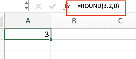
• =ROUNDUP(3.2, 0) results in 4

• =ROUND(3.2, 0) results in 3

Rounding Down in Excel

The ROUNDDOWN function always rounds numbers down. Its syntax mirrors ROUND and ROUNDUP:

=ROUNDDOWN(number, num_digits)

To use ROUNDDOWN:

Step 1: Select your result cell

Step 2: Enter the ROUNDDOWN formula

• Type =ROUNDDOWN(

• Input your number or cell reference.
• Add a comma and specify decimal places.
• Close the parenthesis.

Step 3: Press Enter

• Your number will be rounded down to the specified decimal places.

ROUNDDOWN is preferable when you need to consistently round down, regardless of the decimal value. For instance, in inventory management, you might round down fractional units to ensure you’re not overstating stock levels.

Excel Rounding for Financial Calculations

Precise rounding is crucial in finance to ensure accuracy in calculations and reports. Here’s how to use ROUND for currency calculations:

Step 1: Format your cells for currency

• Select the cells you’ll be working with.
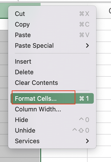
• Right-click and choose ‘Format Cells.‘

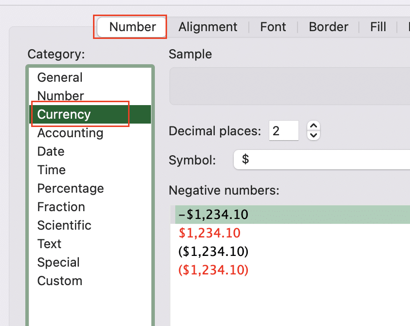
• Select ‘Currency’ under the ‘Number’ tab.

Step 2: Apply the ROUND function

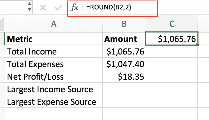
• In a new cell, type =ROUND(

• Select the cell with your financial value.
• Type ,2)

• Press Enter.

For handling large financial datasets with ROUND:

Step 1: Select the range of cells with your financial data

Step 2: Enter the ROUND formula

• In the formula bar, type =ROUND(
• Select the entire range of cells.

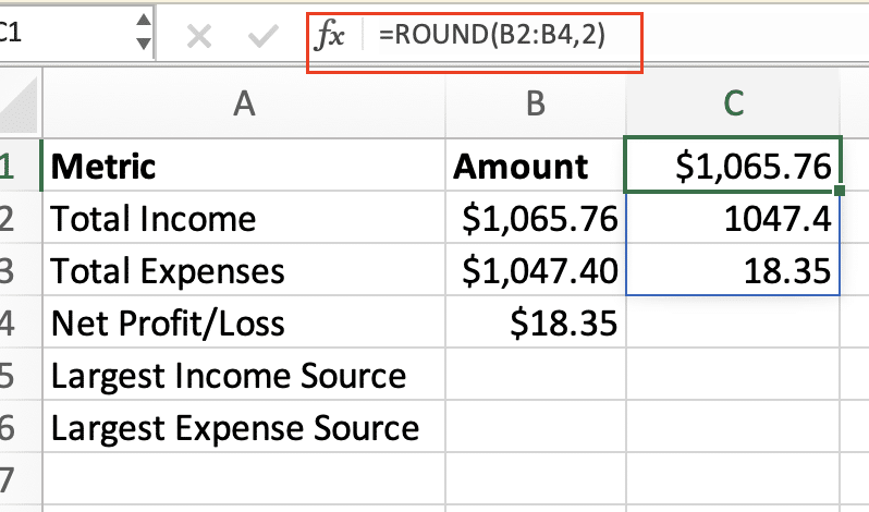
• Type ,2)

Step 3: Press Ctrl + Shift + Enter

• This applies the formula to the entire range as an array formula.

How to Get Excel to Round Correctly

To ensure consistent rounding across your workbook:

Step 1: Access Excel Options

• Click ‘File’ > ‘Options’.

Step 2: Navigate to Advanced settings

• Select ‘Advanced’ in the left pane.

Step 3: Set precision as displayed

• Under ‘When calculating this workbook‘, check ‘Set precision as displayed‘.

Step 4: Click ‘OK’ to apply changes

This setting ensures that Excel uses the displayed value for all calculations, avoiding rounding errors.

To address common rounding errors:

1. Use ROUND in intermediate calculations, not just final results.
2. Be consistent with the number of decimal places used throughout your workbook.
3. Use ROUNDUP or ROUNDDOWN when appropriate, rather than always relying on ROUND.

Practical Applications of ROUND in Data Analysis

ROUND is valuable for data normalization, helping to standardize data to a consistent scale. Here’s how to apply it:

Step 1: Identify your data range

Step 2: Apply ROUND to normalize

• In a new column, use =ROUND(

• Reference your data cell.
• Specify a consistent number of decimal places.
• Close the parenthesis.

Step 3: Copy the formula down the column

• This normalizes your entire dataset to the same decimal precision.

For statistical calculations, ROUND can be combined with functions like AVERAGE, STDEV, or MEDIAN:

=ROUND(AVERAGE(A1:A100),2) =ROUND(STDEV(B1:B50),3) =ROUND(MEDIAN(C1:C75),1)

In data visualization, ROUND can help simplify data for clearer presentation:

Step 1: Select your data range

Step 2: Apply ROUND to each cell

• Use =ROUND( followed by the cell reference and desired decimal places.

Step 3: Create your chart or graph

• Use the rounded values for a cleaner, more digestible visualization.

Wrap-Up: Mastering Excel’s ROUND Function

Excel’s ROUND function is essential for precise data handling. Practice with various decimal places and combine it with other functions to enhance your spreadsheet skills.

Ready to take your Excel skills to the next level? Get started with Coefficient to seamlessly integrate your spreadsheets with live data from various business systems. Start your journey with Coefficient today.