
The PV (Present Value) function in Excel helps calculate the current worth of future payments or investments. Whether you’re evaluating loans, investments, or retirement plans, understanding how to use the PV function effectively is crucial for making informed financial decisions.
How to Use the PV Function in Excel
The PV function calculates the present value of an investment based on future payments and a constant interest rate. Here’s the basic syntax:
=PV(rate, nper, pmt, [fv], [type])
Where:
- rate: Interest rate per period
- nper: Total number of payment periods
- pmt: Payment made each period
- [fv]: Future value (optional)
- [type]: When payments are due (0 for end of period, 1 for beginning)
Let’s break this down with practical examples.
Calculate Present Value of a Single Future Payment
Step 1: Set up your worksheet Create a new Excel worksheet with these column headers:
- Rate (per period)
- Number of periods
- Payment
- Future value
- Payment timing
Step 2: Input the following example
|
Rate |
Periods |
Payment |
Future Value |
Type |
Present Value |
|---|---|---|---|---|---|
|
5% |
3 |
0 |
$10,000 |
0 |
=PV(A2,B2,C2,D2,E2) |
This calculates the present value of $10,000 received in 3 years at 5% interest rate.
Result: -$8,638.38 (negative because it represents an investment)

Example 1: Investment Valuation
=PV(5%/12, 36, 0, 10000, 0)
This calculates how much you need to invest today to have $10,000 in 3 years with monthly compounding.

Find Present Value of Regular Payment Streams
Step 1: Calculate monthly loan payments
|
Rate (Annual) |
Periods |
Monthly Payment |
Future Value |
Type |
Present Value |
|---|---|---|---|---|---|
|
6% |
360 |
-1,000 |
0 |
0 |
=PV(A2/12,B2,C2,D2,E2) |
This shows how much you can borrow if you can afford $1,000 monthly payments for 30 years.

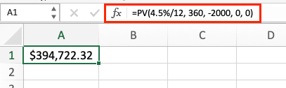
Example 2: Mortgage Calculation
=PV(4.5%/12, 360, -2000, 0, 0)

Stop exporting data manually. Sync data from your business systems into Google Sheets or Excel with Coefficient and set it on a refresh schedule.
Get Started
This calculates how much house you can afford with $2,000 monthly payments over 30 years at 4.5% annual interest.
Essential PV Function Parameters
Rate Parameter
- Must be expressed per period
- For monthly payments with annual rate: divide by 12
- Example: 6% annual rate for monthly calculations = 6%/12 = 0.5%
Number of Periods (nper)
- Must match the rate period
- For 5-year monthly loan: 5 * 12 = 60 periods
- Example: 30-year mortgage = 360 periods
Payment (pmt)
- Must be consistent amount
- Negative if you’re paying out
- Positive if you’re receiving
Working with Different Payment Frequencies
Example 3: Converting Annual to Monthly Payments
|
Annual Rate |
Years |
Annual Payment |
Monthly Rate |
Monthly Periods |
Monthly Payment |
|---|---|---|---|---|---|
|
7.2% |
5 |
-12,000 |
=A2/12 |
=B2*12 |
=C2/12 |

Real-World Applications
Loan Amount Calculation
To find maximum loan amount with:
- Monthly payment: $1,500
- Annual interest: 4.8%
- Term: 15 years
=PV(4.8%/12, 15*12, -1500, 0, 0)

Investment Planning
To calculate needed investment for retirement:
- Target amount: $500,000
- Years until retirement: 25
- Annual return: 6%
=PV(6%, 25, 0, 500000, 0)

Retirement Planning
To determine present value of future retirement payments:
- Monthly withdrawal: $3,000
- Years of retirement: 20
- Expected return: 5%
=PV(5%/12, 20*12, -3000, 0, 0)

Next Steps
Now that you understand how to use Excel’s PV function effectively, you can apply these calculations to your financial planning and analysis. For more advanced financial modeling and real-time data integration, consider using Coefficient to connect your spreadsheets directly to your financial data sources.
Start automating your financial calculations with Coefficient today
<meta_description> SERP Title: Master Excel’s PV Function: Calculate Present Value Like a Pro Meta Description: Learn to use Excel’s PV function for precise present value calculations. Complete guide with real examples for loans, investments & retirement planning. </meta_description>


