The OFFSET function in Excel enables users to create flexible, dynamic ranges that automatically adjust as data changes. This powerful function returns a reference to a range that’s a specified number of rows and columns from a starting point. Whether you need to build dynamic reports, create flexible charts, or automate range selection, OFFSET provides the foundation for advanced Excel solutions.

Create Dynamic Ranges with Excel’s OFFSET Function

Let’s start with a practical example to understand how OFFSET works in real-world scenarios.

Set Up Sample Data

First, create a sample dataset to work with:

Month	Sales
Jan	1200
Feb	1500
Mar	1800
Apr	2100
May	2400

Basic OFFSET Formula Structure

The OFFSET function uses five parameters:

OFFSET(reference, rows, cols, [height], [width])

Where:

• reference: Starting cell or range
• rows: Number of rows to offset (positive = down, negative = up)
• cols: Number of columns to offset (positive = right, negative = left)
• height: Optional height of returned range
• width: Optional width of returned range

Step-by-Step: Create Your First OFFSET Formula

1. SELECT your starting cell (e.g., A2)
2. ENTER the formula:

=OFFSET(A2,1,0)

1. PRESS Enter to see the result

This formula returns the value one row below A2.

Build Advanced Excel Reports Using OFFSET

Return Data from Different Rows and Columns

Let’s create a dynamic reference that adjusts based on user input:

1. CREATE a cell for user input (e.g., G1)
2. LABEL it “Months to Show”
3. ENTER the formula:

=OFFSET(A2,0,0,G2,2)

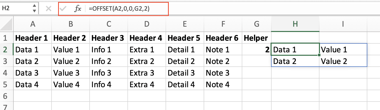
This creates a range that automatically adjusts based on the value in G1.

Create Flexible Range References

To make your ranges more dynamic:

1. OPEN Name Manager (Formulas tab)

1. CREATE a new named range
2. ENTER the formula:

=OFFSET(Sheet1!$A$2,0,0,COUNTA(Sheet1!$A:$A)-1,2)

This named range will automatically expand as new data is added.

Combine OFFSET with Other Excel Functions

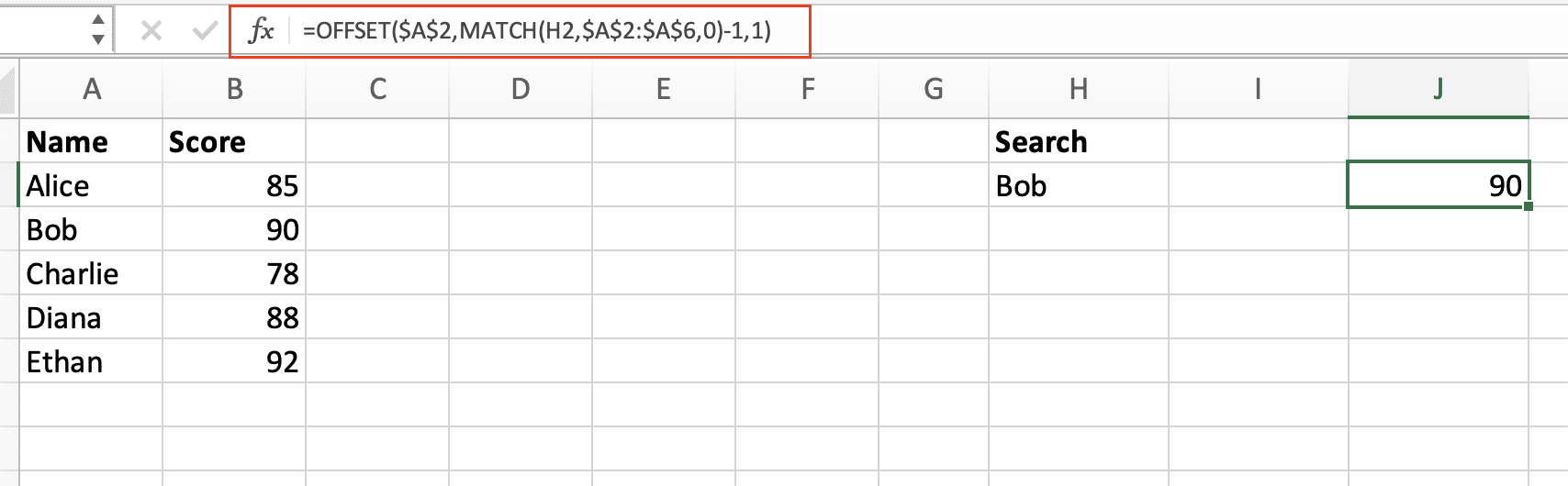
Use OFFSET with MATCH for Flexible Lookups

Create dynamic lookups that adapt to changing data:

1. SET UP a search value in cell H1
2. ENTER the formula:

=OFFSET($A$2,MATCH(H1,$A$2:$A$6,0)-1,1)

This returns the corresponding value from the second column

.

Replace OFFSET with INDEX When Needed

While OFFSET is powerful, INDEX can be more efficient for certain tasks:

Function	Volatile	Performance	Use Case
OFFSET	Yes	Slower	Dynamic ranges
INDEX	No	Faster	Static lookups

Common OFFSET Applications in Excel

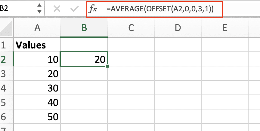
1. Calculate Moving Averages:

=AVERAGE(OFFSET(A2,0,0,3,1))

1. Create Dynamic Charts:

• SELECT your data range
• CREATE a named range using OFFSET
• REFERENCE the named range in your chart

1. Reference Last N Entries:

=OFFSET(A2,COUNTA(A:A)-5,0,5,1)

This formula returns the last 5 entries in column A.

Taking Your OFFSET Skills Further

The OFFSET function opens up countless possibilities for dynamic Excel solutions. Practice these techniques with your own data to master them. Remember to:

• Start with simple formulas
• Test thoroughly before implementing in production
• Consider performance implications for large datasets

Ready to take your Excel reporting to the next level? Coefficient helps you automate your spreadsheet workflows and keep your data fresh with live connections to 50+ business systems. Get started with Coefficient to transform your Excel experience today.