
The OFFSET formula in Excel is a powerful tool that helps you reference cells or ranges by specifying a starting point and moving a certain number of rows and columns. This makes managing large datasets or tables much easier, as you can create formulas that automatically adjust as your data changes.
In this article, you’ll learn how to use the OFFSET formula in Excel and discover practical examples to help you get started. Get ready to enhance your spreadsheet skills and simplify your data management!
Understanding Syntax Of The OFFSET Formula In Excel
The syntax of the OFFSET formula in Excel is: =OFFSET(reference, rows, cols, [height], [width])
Let’s examine each argument in a little more detail:
- The reference argument can be a single cell or a range of adjacent cells from which you desire to OFFSET the output.
- The rows argument is a number that specifies how many rows up/down the function should move from the reference. This number can be positive (for moving down) or negative (for moving up).
- The cols argument is a number that specifies how many columns left/right the function should move from the reference. This number can be positive (for moving right) or negative (for moving left)
- The height argument is optional and defines the number of rows to output. Not specifying it makes it default to the number of rows in reference.
- The width argument is optional and defines the number of columns to output. Not specifying it makes it default to the number of rows in reference.
We’ll demonstrate the OFFSET formula in Excel with a couple of simple examples.
Example: Returning A Single Cell Or Range From A Range Of Cells
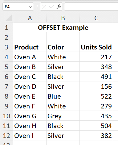
Let’s say you have a data set that looks like this:
To get the value of cell B8 (“Blue”), you can use cell A3 as the reference and define the formula as: =OFFSET(A3,5,1)
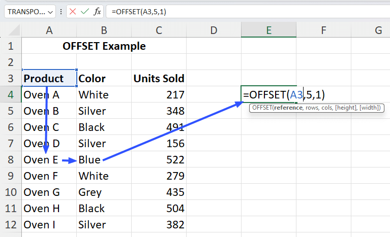
This returns the value of the cell that is 5 rows down and 1 column to the right of the reference cell, A3.
But that doesn’t accomplish anything, does it?
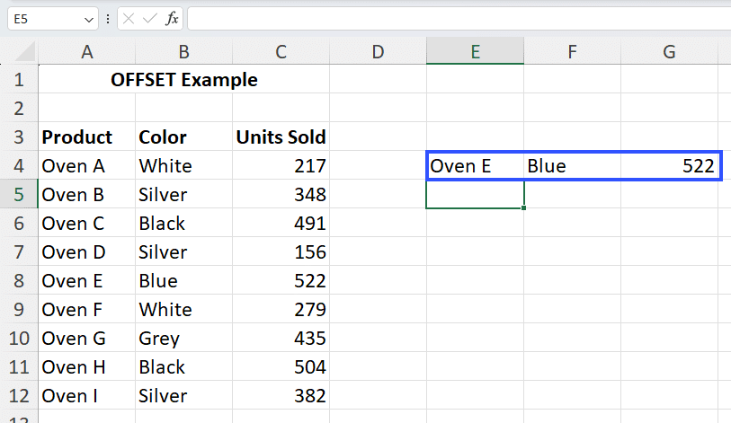
What if you wanted to display all the values (Product, Color, Units Sold) of a single product? You can use the OFFSET function to return those values by writing the formula: =OFFSET(A3:C3,5,0)
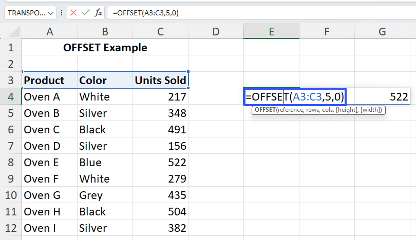
This returns a range of cells that is 5 rows down and 0 columns from the reference range A3:C3 and is 1 row high, 3 columns wide (as that’s the dimension of the reference range).
You can also define the OFFSET function to return a range that is smaller or bigger than the reference range but not 0. You’d do it by specifying the height and width arguments, like so: =OFFSET(A3:C3,3,0,3,2)

This returns a 3×2 range of cells that is 3 rows below and 0 columns from the reference range A3:C3.
But, you may be asking, why use the OFFSET formula in Excel instead of just copying data from the required range?
A valid question, which we’ll answer in the next section.
How To Use OFFSET Formula For Dynamic Calculations
When you have a static data set, you can use regular functions like SUM, AVERAGE, MIN, MAX, etc., as intended. But if rows/columns are being added or deleted from the sheet dynamically (maybe because it’s connected to software that’s importing live data), defining a fixed range in these operations won’t give you the result you want.
That’s when you use the OFFSET formula in Excel to perform calculations on dynamic data sets. Let’s take a look at some practical examples to make the use of the OFFSET formula in Excel topic clearer.
Example #1: Combining OFFSET With SUM, AVERAGE, MAX, And MIN For Dynamic Range Calculations
Let’s say you’re pulling/copying data from your sales dashboard into an Excel spreadsheet to calculate the total sales of your products.
The sales dashboard is updated every week, so if you use the SUM function, you’ll have to update your SUM formula every time new sales data is added.
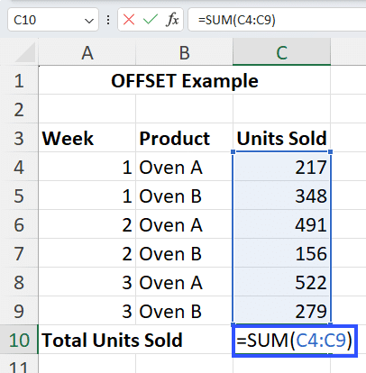
Instead, you could combine OFFSET with the SUM function to make the function dynamic so it updates every time new data is added. The formula for that will be: =SUM(C4:OFFSET(C10,-1,0))
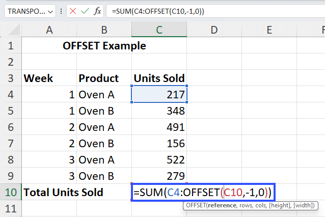
This will return the value 2013, which is the sum of all the values from C4 to C9 (which is 1 row above and 0 columns from the reference cell C10).
Now, when new data is inserted between rows 9 and 10, the formula will recalculate to give you the correct total.
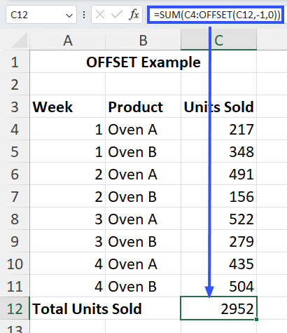
And you didn’t even have to touch the cell with the formula for this as OFFSET takes a dynamic cell reference!
You can combine the OFFSET formula in Excel with the AVERAGE, MAX, And MIN functions in a similar manner.
Example #2: Combining OFFSET With COUNT For Dynamic Range Calculations
In the previous example, you defined the starting point of the range manually (i.e., C4) and the ending point of the range with the OFFSET function.
However, if you want to insert the previous month’s data above C4, the formula in the previous example wouldn’t return the correct value. In such cases, you can combine OFFSET with the COUNT function to make the function completely dynamic.
The formula would look like this: =SUM(OFFSET(C3,1,0,COUNT(C:C)))
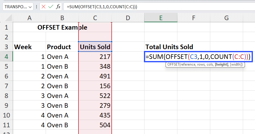
This will return the sum of all the numerical values in column C.
Note: We didn’t place the cell containing the formula in column C as this would result in a warning about the formula not working correctly.

Example #3: Using OFFSET With Drop-down Lists For Dynamic Range Calculations
You can also use the OFFSET formula in Excel to do on-the-fly calculations by combining it with a drop-down list. Let’s see an example.
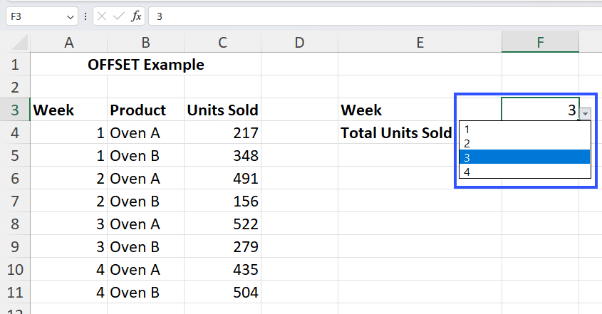
Let’s say you create a drop-down list where you can select the week, and you want to see the total units sold for each week. We’ll calculate this for week 3 in this example.
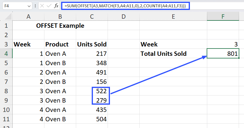
You’ll need to use the formula: =SUM(OFFSET(A3,MATCH(F3,A4:A11,0),2,COUNTIF(A4:A11,F3)))
Let’s break this down:
- You want to calculate the sum of all units sold in week 3, so you want the OFFSET function to return an array containing the units sold of each product in that week.
- So, the reference argument for OFFSET will be A3, which is the first cell in the data set.
- Next, the rows argument for OFFSET needs to be 2, as there are two products. But what if there were 3 or 4 products? Or what if the number of products in each week was different?
Hence, we need to make the rows argument dynamic by checking how many cells match the criteria in cell F3. So, you use MATCH(F3,A4:A11,0) to define it. - You want the SUM function to calculate the total units sold, which is 2 columns to the right of the reference cell A4. So the columns argument for OFFSET becomes 2.
- Finally, you want the OFFSET function to return an array of n rows that match the criteria in cell F3. So, you use COUNTIF(A4:A11,F3) to define the height argument.
- You can skip the width argument as you only want the result to be one column wide.
The result of this formula is the sum of the units sold of each product in week 3.
Example #4: Applying The OFFSET Formula in Excel For Dynamic Chart Ranges
If you’re visualizing data in a table using charts, the OFFSET function can offer a way to create dynamic chart ranges. To accomplish this, you need to use the OFFSET function to return a subset of the data from the table and base the chart on this returned array.
Let’s say you have the same data set as the previous example, and you want to display a chart of all the data until week 3. You’d use the formula: =OFFSET(A3,1,0,MATCH(3,Table4[Week],0)+1,COLUMNS(Table4))

Stop exporting data manually. Sync data from your business systems into Google Sheets or Excel with Coefficient and set it on a refresh schedule.
Get Started
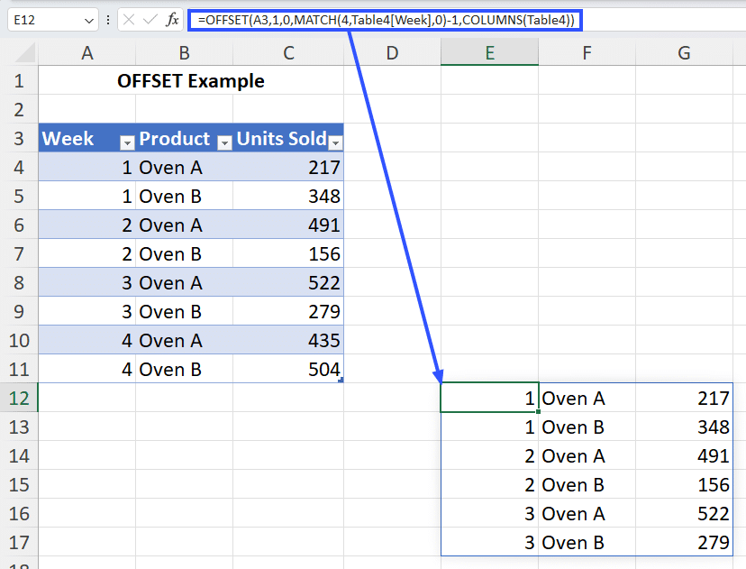
This would return all the values in the table (named Table 4) from weeks 1-3.
Let’s break down the formula to see how we achieved this:
- For the reference argument, we use A3, which is the first cell in the table.
- The row argument is 1 since we need to view the data starting with row 4.
- The columns argument is 0 since we don’t need to move any columns to the left or right.
- For the height argument, we used the MATCH function to return the position of the first cell containing 4 in the “Week” column and subtracted 1 from it.
- For the width argument, we counted the number of columns in the table using the COLUMNS function.
Now, you can select the cell with the OFFSET formula in EXCEL and insert a chart without having to select a specific range in the original table.
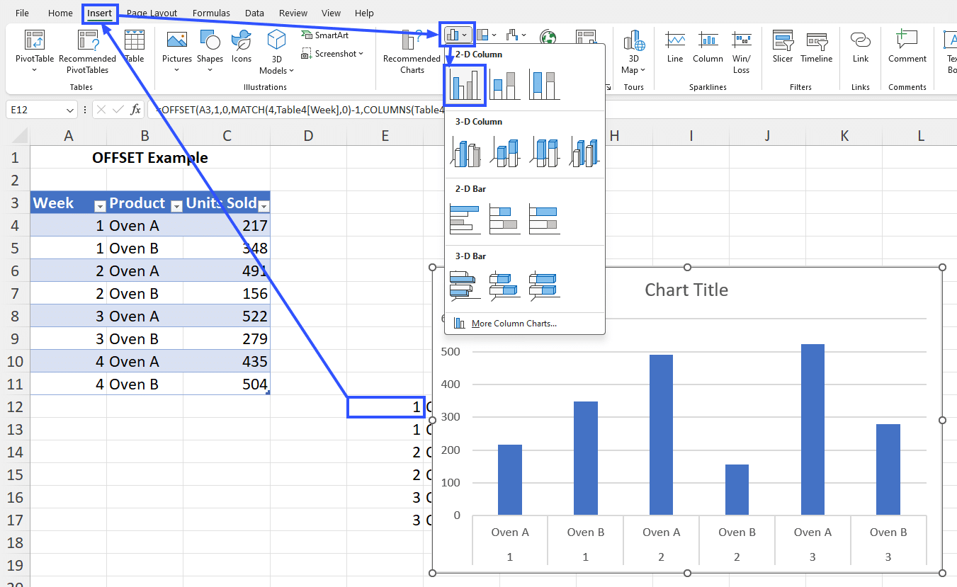
Any changes you make in the table will be reflected in the chart as well.
Example #5: Using OFFSET With VLOOKUP And HLOOKUP Functions For Versatile Lookup
The most common limitation of the VLOOKUP and HLOOKUP functions is their inability to look for values on any column other than the leftmost column/topmost row in the table. However, you can overcome this limitation by creating a dynamic reference to the table using the OFFSET function.
We’ll use the same data set as in the previous example and try to find the product name whose units sold match the value in cell F5 by using the formula: =VLOOKUP(F4, Table4,-1)
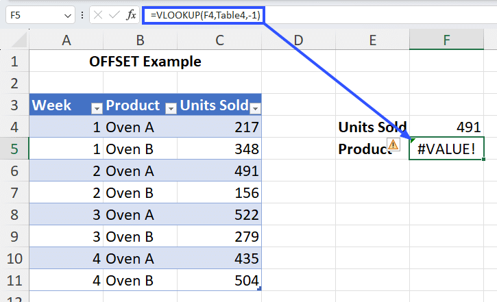
This will return the #VALUE! error as the col_index_num argument is -1.
To overcome this issue, we can use OFFSET to create dynamic references to the “Product” and “Units Sold” columns such that the lookup_value is located in the leftmost column of the table_array.
So, you use the formulas as follows:
- Cell E4: =OFFSET(A4,0,2,COUNT(A:A))
- Cell F4: =OFFSET(A4,0,1,COUNT(A:A))
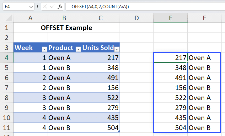
This will result in the values in the “Product” and “Units Sold” columns appearing in an array with switched positions.
Now, you can use VLOOKUP on this new array (E4:F11) by using the formula: =VLOOKUP(I3,E4:F14,2,FALSE)
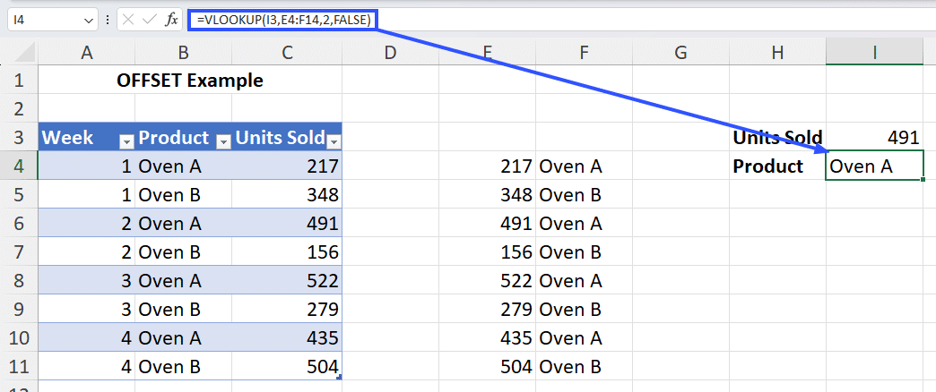
This will result in the function finding the value in cell I3 in the array extracted using the OFFSET function and displaying the value in the second column of the array.
It seems like a roundabout way of doing things, but it works. That’s the benefit of using the OFFSET formula in Excel, but it’s not without its shortcomings.
Practical Example #1:
You have a list of monthly sales figures in column B, and this list is updated monthly. You want to create a dynamic formula that always calculates the average of the latest 5 months of sales.
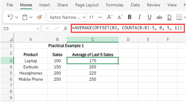
Explanation of the Formula: OFFSET(B3, COUNTA(B:B)-5, 0, 5, 1)
- A1: The reference point from where the OFFSET starts.
- COUNTA(A): Counts the number of non-empty cells in column A. This gives us the total number of entries.
- COUNTA(A)-5: Calculates the row number for the starting point of the last 5 entries.
- 0: No offset in columns, i.e., stay in column A.
- 5: The height of the range, which is 5 rows.
- 1: The width of the range, which is 1 column.
Well, how does it work? As new sales figures are added to column B, the COUNTA(B:B) part of the formula updates automatically, ensuring that the OFFSET formula always points to the last 5 entries. Also, the AVERAGE function then calculates the average of these 5 values.
Common Challenges In Using OFFSET And How To Overcome Them
Here are some common issues you might encounter when using the OFFSET formula in Excel:
- #REF! Error: This error occurs when the reference specified in the OFFSET function is invalid. To fix this, ensure that the reference cell or range exists and is valid. Check for typos in cell references and adjust them accordingly.
- #VALUE! Error: This error usually indicates that the formula is trying to perform a calculation with incompatible data types. To resolve this, make sure that the input values or references in the OFFSET function are of the correct data type (e.g., numbers instead of text).
- Difficulty Reviewing And Debugging OFFSET Formulas: Due to the dynamic nature of the OFFSET formula in Excel and its potential impact on cell references, it can be challenging to review and debug errors. To help with this, try using Excel’s Evaluate Formula tool, double-check cell references, and thoroughly familiarize yourself with the OFFSET function’s behavior by testing with different inputs.
- Negative Performance Impact On Excel: The OFFSET function is volatile, meaning it recalculates every time there is a change in the worksheet. This can slow down the recalculation process, especially in large data ranges. The performance can decrease further when OFFSET is used within array formulas or has multiple instances of the function. To deal with this issue, you’ll have to try to minimize the number of times you use the OFFSET function.
To overcome these limitations of the OFFSET function, consider using alternative functions.
Alternatives To The OFFSET Function in Excel
There are several alternative functions to OFFSET that you can use for dynamic references in Excel. Here are some commonly used alternatives:
- The INDEX and MATCH functions can be combined to dynamically reference cells based on specific criteria.
- The INDIRECT function also allows you to create references to cells indirectly based on a text string, but it is also a volatile function.
- You can also use VLOOKUP and HLOOKUP functions to search for a value in a table and return a corresponding value in the same row (VLOOKUP) or column (HLOOKUP).
- By structuring your Excel Tables And Pivot Tables appropriately, you can create dynamic cell references that function similarly to OFFSET.
Having discussed the alternatives, let’s wrap up the discussion on the OFFSET function
Using The OFFSET Function In Excel
Imagine mastering the OFFSET formula in Excel. With the guid above, you’ll be able to tackle and possess the ability to create dynamic cell references that make your calculations more flexible and efficient.
Picture this: your database or CRM is linked to Excel, updating your data set regularly. Instead of wasting time on repetitive operations and tedious manual data manipulation, you can streamline your workflow and let Excel handle the heavy lifting. Learning to perform calculations on dynamic ranges isn’t just important—it’s a game-changer for anyone looking to stay ahead in data management.
So, say hello to Coefficient, the leading spreadsheet automation tool that connects to any data source, imports live data, and automates spreadsheet workflows. Get started today and make your tasks easier by using the OFFSET formula in EXCEL.


