Using The MAXIFS Function In Excel [Step-by-Step Guide With Examples]

It is often overwhelming to try to find your way through the numerous functions of Excel, but it is worth the effort since it can significantly improve your data-handling abilities. Just think about the possibility of identifying the greatest value in a given array of values within a few seconds, provided that you have certain criteria in mind—this is where the MAXIFS function comes in handy. Whether you are a Data Analyst, a CA, or a regular user who wants to make his/her work easier, knowing how to use MAXIFS can make a big difference.

The MAXIFS function is specifically used to find the largest value in a set of cells that meets one or more conditions.

Here, you will find a step-by-step guide on how to use the MAXIFS function in Excel, along with examples to illustrate its capabilities. Well, it is time to start exploring this powerful Excel tool and reveal its secrets!

What Is The MAXIFS Function?

The MAXIFS function finds the highest value in a range based on one or more conditions by aiding in finding the highest data point that meets certain conditions from a large set of data. MAXIFS allows the specification of various conditions and instant recognition of peaks in certain conditions, which makes data analysis and decision-making processes much more accessible.

Understand The MAXIFS Function: Syntax And Parameters

Here is the function syntax followed by a detailed breakdown of each parameter, including examples:

=MAXIFS(max_range, criteria_range1, criteria1, [criteria_range2, criteria2], …)

The formula consists of several components that work together to perform the desired MAXIFS function. Let’s understand each component in detail:

1. ‘max_range’ – This is the range of cells from which the maximum value will be determined. It is the primary set of data where Excel looks for the highest value based on the given criteria.
2. ‘criteria_range1, criteria_range2,’ etc. – These are the ranges of cells where the criteria are applied. Each ‘criteria_range’ corresponds to a criterion (criteria1, criteria2, etc.) that defines what cells in the ‘max_range’ should be considered for finding the maximum value.
3. ‘criteria1’, ‘criteria2’, etc. – These are the conditions that the corresponding criteria_range must meet in order for the cells in max_range to be considered. Conditions can be numeric, text (such as names or labels), or date values, and they can include logical operators (like >, <, =, etc.).

Example Formula:

=MAXIFS(A1:A10, B1:B10, “Electronics”, C1:C10, “North”)

In this formula:

• A1:A10 is where the sales figures are stored (‘max_range’).
• B1:B10 is the range that contains the product categories (criteria_range1).
• “Electronics” specifies the condition that the category must be “Electronics” (criteria1).
• C1:C10 is the range that contains the regions (criteria_range2).
• “North” specifies the condition that the region must be “North” (criteria2)

This formula will review the sales figures in the range A1:A10, but only consider those figures where the corresponding cells in B1:B10 are “Electronics,” and those in C1:C10 are “North”. The result will be the highest sales figure meeting these conditions.

Video Tutorial

Check out the tutorial below for a complete video walkthrough!

How To Use The MAXIFS Function With Single And Multiple Criteria

The ‘MAXIFS’ function in Excel is designed to return the maximum value in a range based on one or more conditions. Here’s a detailed guide on how to use the ‘MAXIFS’ function with a single criterion, including a practical example.

Single Criterion

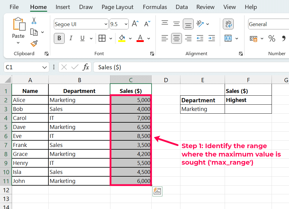
Step 1: Identify the range where the maximum value is sought (‘max_range’)

In our example, the ‘max_range’ is the column containing the sales figures. In an Excel sheet, if this data starts from cell C2 to C11, then ‘max_range’ is C2:C11.

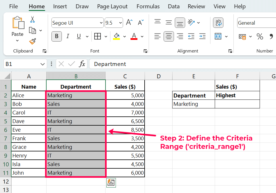
Step 2: Define the Criteria Range (‘criteria_range1’)

The criteria_range1 is the column that contains the data against which the criteria will be checked. In our case, since we are looking for sales in a specific department, ‘criteria_range1’ will be the Department column, B2:B11.

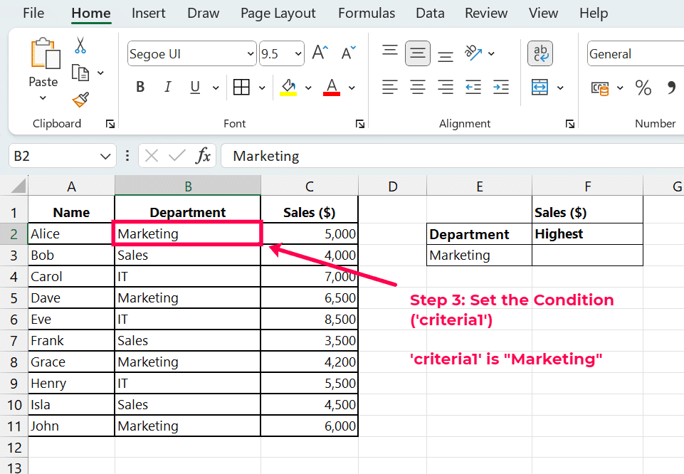
Step 3: Set the Condition (‘criteria1’)

The criteria1 defines the condition that must be met within the ‘criteria_range1’. Suppose we want to find the maximum sales in the “Marketing” department. Then, ‘criteria1’ is “Marketing”.

Step 4: Apply the MAXIFS Function

Insert the MAXIFS function in a cell where you want to display the result. Based on our setup, the function will look like this:

=MAXIFS(C2:C11, B2:B11, “Marketing”)

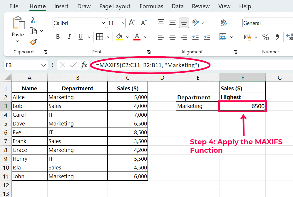
Step 5: Interpret the Results

After entering the formula, Excel will display the maximum sales figure for the Marketing department. According to our dataset, Dave achieved the highest sales in Marketing, $6,500.

Multiple Criteria

To elaborate on using the ‘MAXIFS’ function in Excel with multiple criteria, we’ll walk through an example step-by-step. This function is particularly useful for finding the maximum value within a dataset that meets specific conditions. Here’s how you can set up and utilize this function effectively:

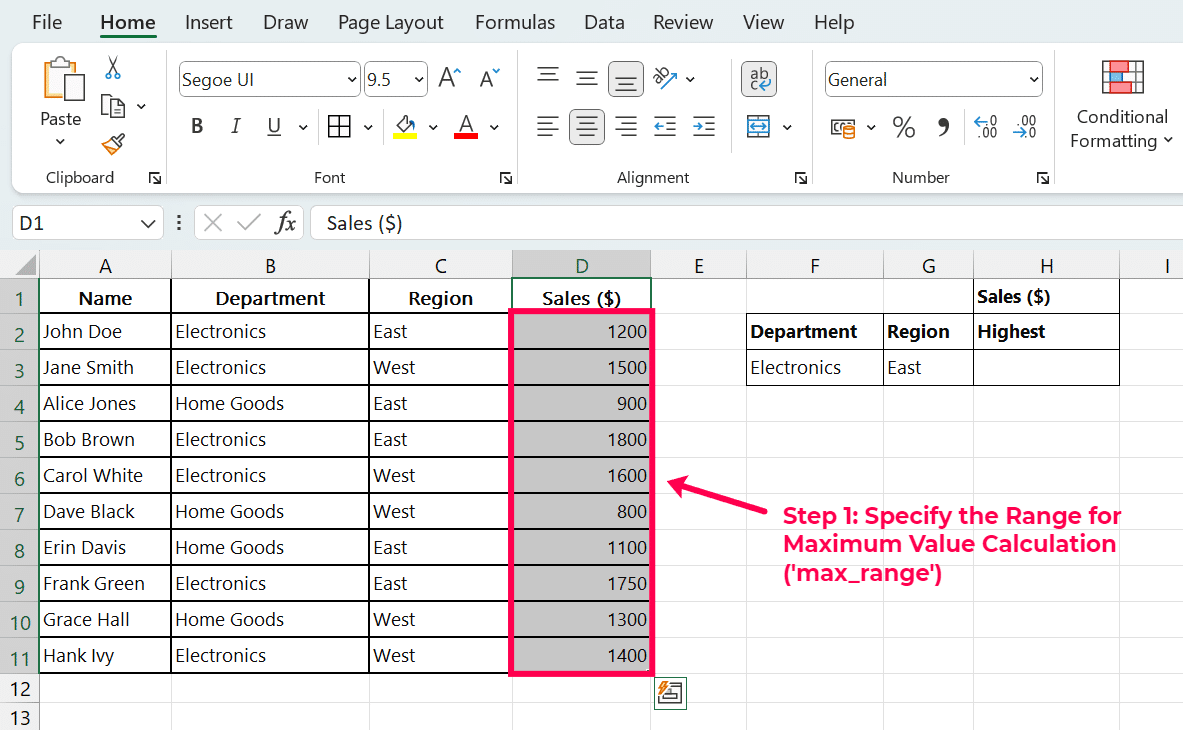
Step 1: Specify the Range for Maximum Value Calculation (‘max_range’)

To begin, specify the range where the maximum value should be calculated. In this case, you want to calculate the maximum sales amount. Therefore, the ‘max_range’ will be the Sales ($) column in your dataset.

Step 2: Define Multiple Criteria Ranges (‘criteria_range1’, ‘criteria_range2’, etc.)

Define the criteria ranges that will be used to filter the data. Here, ‘criteria_range1’ is the Department column, and ‘criteria_range2’ is the Region column.

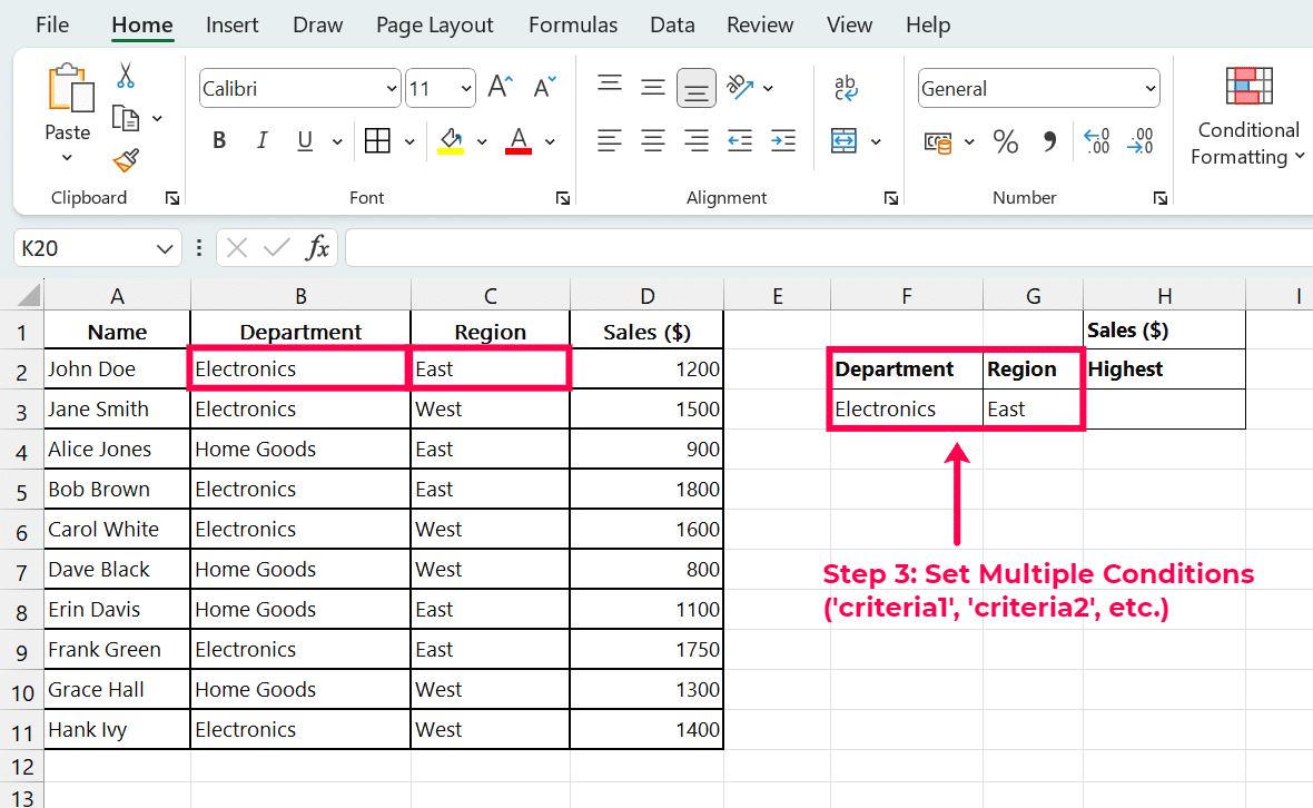
Step 3: Set Multiple Conditions (‘criteria1’, ‘criteria2’, etc.)

Set the conditions for each criteria range. ‘criteria1’ might be “Electronics”, meaning you are interested in finding the maximum sales in the Electronics department. ‘criteria2’ might be “East”, focusing only on sales in the Eastern region.

Step 4: Apply the MAXIFS Function with Multiple Criteria

Combine the ranges and criteria in the MAXIFS function to calculate the maximum sales for Electronics in the East region. The formula will look like this:

=MAXIFS(D2:D11, B2:B11, “Electronics”, C2:C11, “East”)

This formula tells Excel to find the maximum value in cells D2 to D11 (Sales column) where cells B2 to B11 (Department column) equal “Electronics” and cells C2 to C11 (Region column) equal “East”.

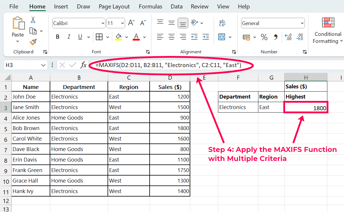
Step 5: Interpret the Results

After applying the ‘MAXIFS’ function, Excel will display the highest sales figures from the electronics department in the East region. Analyze this result within the context of your data to make informed decisions or further inquiries.

In our example, it has returned $1800, indicating that Bob Brown has the highest sales figure under the specified conditions.

Advanced Tips And Tricks

Here are the advanced tips and tricks for using the MAXIFS function, including integrating it with dynamic ranges and other functions:

Apply MAXIFS with the Dynamic Ranges (employing OFFSET or INDEX).

• Dynamic Range with OFFSET – MAXIFS can be made more flexible when coupled with OFFSET function. This combination makes the range that MAXIFS is searching for the highest value to be dynamic and adjustable. For example, ‘=MAXIFS(OFFSET(A1,0,0,COUNT(A:A1:B100, “>10”)’ searches for the maximum value in the range from A1 to B100, and adjusts the height of the graph based on the number of non-empty cells in column A where corresponding values in column B are greater than 10.
• Dynamic Range with INDEX – INDEX helps us to generate non-consecutive dynamic ranges for MAXIFS function. This method is beneficial because it allows to apply MAXIFS over several non-contiguous ranges. An example is ‘=MAXIFS(INDEX(A:A,1):INDEX(A:A,10), B1:B10, “>5”)’, which finds the maximum value from A1 to A10 where the corresponding values in B1 to B10 exceed 5.

Combine MAXIFS with Other Functions (e.g., IF, AND, OR) for Complex Criteria

• Use AND Logic – Combine MAXIFS with the ability to meet all conditions by using the native MAXIFS functionality to handle multiple conditions. For instance, ‘=MAXIFS(C1:C100, A1:A100, “>200”, B1:B100, “<500”)’ finds the maximum value in C when values in A are higher than 200 AND values in B are fewer than 500.
• Use OR Logic with Array Formulas – To make use of the OR logic which MAXIFS does not offer as a native function, you can use an array formula. For example, ‘=MAX(IF((A1:A100 = “Red”) + (A1:A100 = “Blue”), B1:B100))’ with Ctrl+Shift+Enter is the maximum in B if A is either “Red” or “Blue”.

Automating Tasks and Analyses with MAXIFS in Excel

Automation of repetitive tasks and complex analyses in Excel with MAXIFS can be done in an efficient way. Through setting up numerous requirements, users can automate the process of fetching the top values from large datasets, thus saving time and increasing accuracy.

Integration of MAXIFS with Financial Data Analysis in Excel

In financial data analysis, integrating the MAXIFS feature gives an analytics tool that can be used to locate the highest financial metrics under given conditions. It can be used in Excel and Google Sheets, thus being applicable to different financial models and reports.

Utilizing MAXIFS in Conjunction with VBA for Custom Excel Applications

The custom Excel applications can be further enhanced by the use of MAXIFS with Visual Basic for Applications (VBA) which provides for even more customization and automation. Such integration makes it possible to create custom functions and applications that can process data with great accuracy and complexity.

Debug Common Errors In MAXIFS

Here are some ways to rectify common errors in the MAXIFS function:

• #VALUE! Error: This may happen if the limit arguments are not of the same length or a non-numeric criteria argument is used. Make sure that all the range parameters have identical sizes and that the criteria are properly set according to the data types you’re working with.
• Criteria Mismatch: Errors are generated when the criteria that are specified do not properly match the data type in the range criteria. For example, if numerical criteria are applied to textual data types or vice-versa, then it gives wrong outputs. Be sure to always check that your criteria types match the data types of the ranges they apply to.
• Handling Non-Existence: If the cell does not meet any of the specified criteria, MAXIFS will return an error #N/A. To handle this, you can wrap MAXIFS in an IFERROR function to specify an alternative output, like so: ‘=IFERROR(MAXIFS(D1:D100, C1:C100, “>=10”), “No Valid Data”)’, which will provide a custom message instead of an error.

Practical Examples and Case Studies

Let’s look at some of the cases and examples where the MAXIFS function is used.

• Example 1: To Find the Maximum Sales in a Particular Region

Sales performance is often evaluated by region in businesses with the aim of guiding strategic moves. They apply the MAXIFS function in the spreadsheet to see the highest sales figures in some regions within certain periods. The procedure is to arrange the sales data into rows under the headings of Date, Sales Amount, and Region. The MAXIFS function is used to find the highest sales in a region, say West, using the formula =MAXIFS(B2:B11, C2:C11, “West”) to find top sales in the West region.

This allows for management to identify the areas that are working well, and consider imitating the successful strategies in other places.

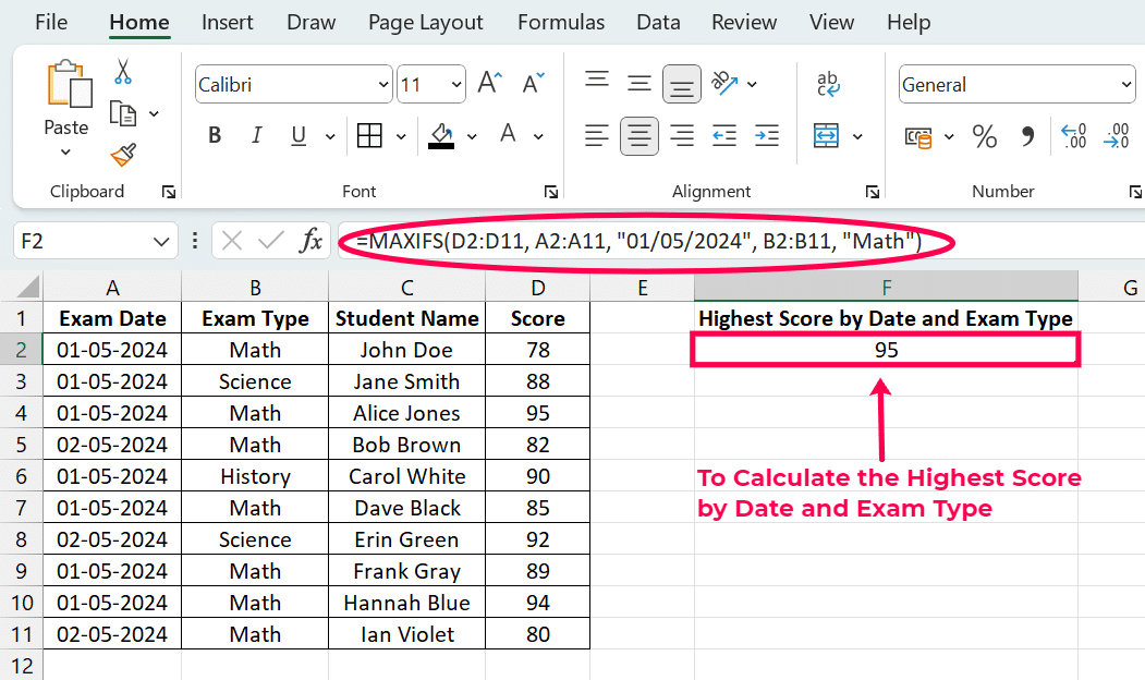
• Example 2: To Calculate the Highest Score by Date and Exam Type

Educational institutions and certification bodies use MAXIFS to identify the highest exam scores by type on that date, helping them to track performance. They format data in columns with Exam Date, Exam Type, Student Name, and Score labels.

The formula =MAXIFS(Score column, Exam Date column, “01/05/2024”, Exam Type column, “Math”) helps to find the best score for a Math exam on May 1, 2024. This approach helps to determine the top scores across the different types of exams, which is an essential component of academic planning and student feedback.

=MAXIFS(D2:D11, A2:A11, “01/05/2024”, B2:B11, “Math”)

• Example 3: How a Business Uses MAXIFS to Streamline Operations

A retail chain applies MAXIFS to improve the efficiency of inventory management and sales strategy, with the objective of maintaining the stock levels of the company’s products at an optimum level across its stores to avoid excessive stocking and ensure availability. The company uses a MAXIFS function to trace the maximum sales of each product by store every month, which allows for optimized inventory management based on actual demand patterns. Formula: =MAXIFS(D2:D11, C2:C11, “January”, A2:A11, “Store B”)

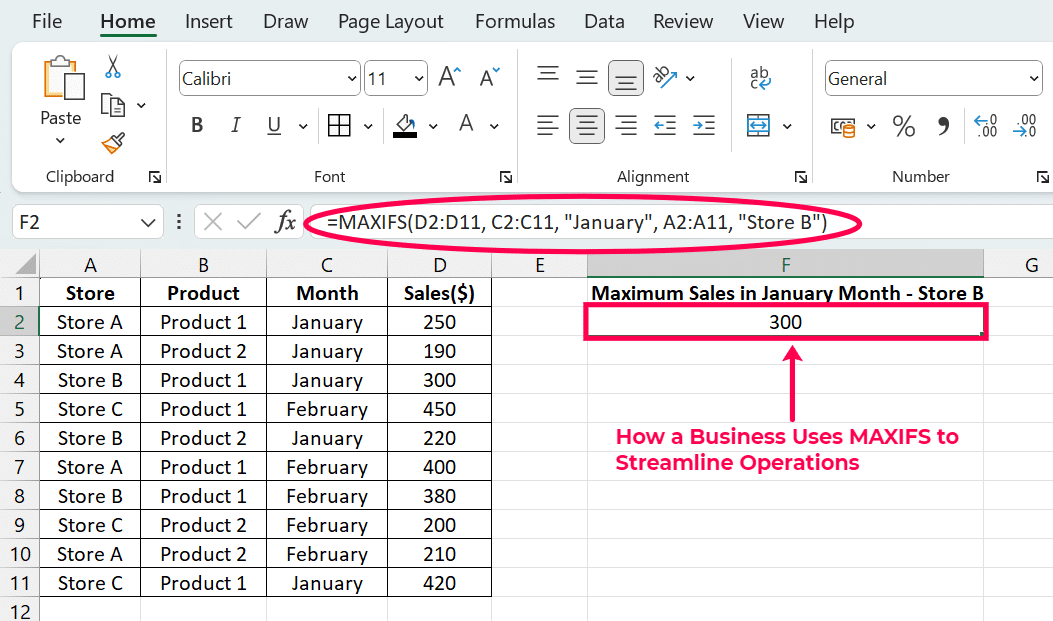
The formula finds the highest sales in Store B during January. It filters the Sales column (D2:D11) by the Month column (C2:C11) for January and the Store column (A2:A11) for Store B, finding that the maximum sales were 300 units. This strategy assists to find the maximum sales of the product by store in a given month.

• Example 4: To optimize Marketing Campaigns

Marketing departments use MAXIFS to appraise the performance of different campaigns through various channels and maximize engagement or conversion rates by campaign type and region. The common case could be an expression like this =MAXIFS(Conversion Rate column, Campaign Type column, “Digital”, Region column, “South”) to find the highest conversion rate for digital campaigns in the Southern region. Formula: =MAXIFS(B2:B11, C2:C11, “Digital”, D2:D11, “South”).

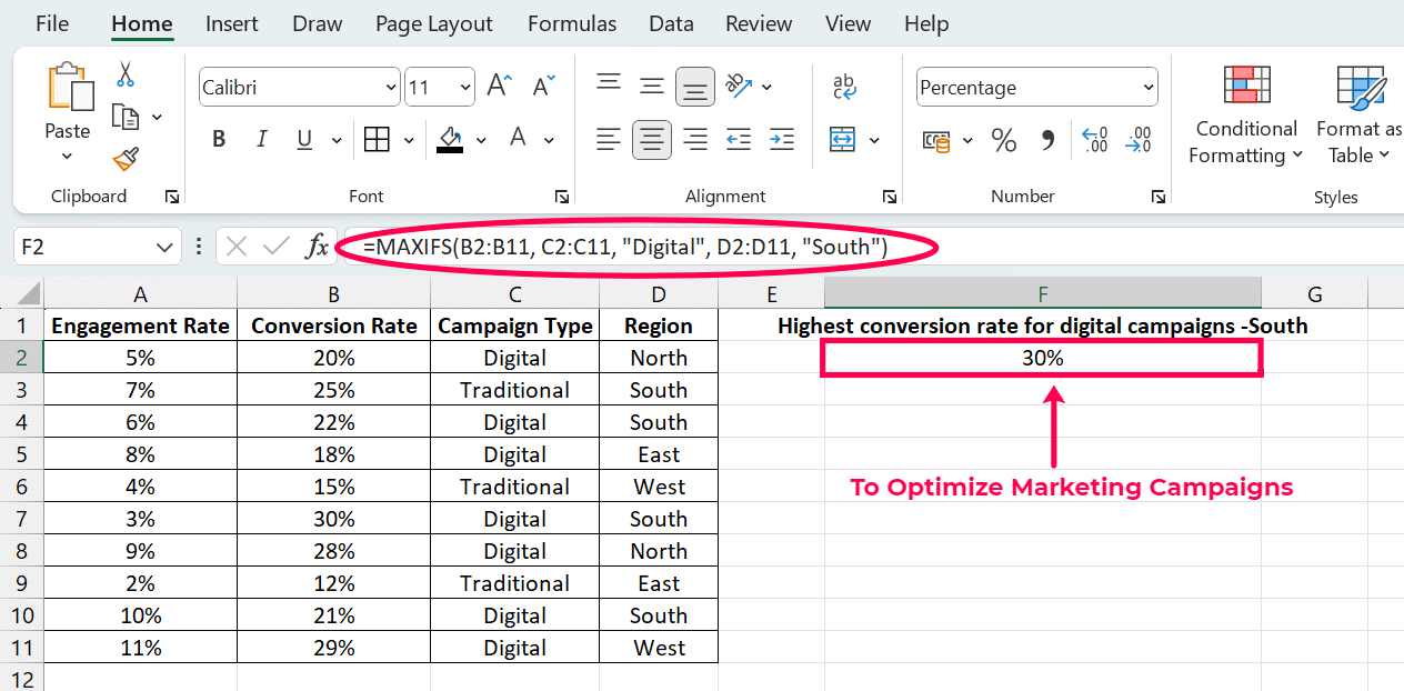
The formula evaluates the Conversion Rate column (B2:B11) to find the maximum value where the Campaign Type column (C2:C11) equals “Digital” and the Region column (D2:D11) equals “South”. The highest conversion rate for digital campaigns in the Southern region is 30%. This analysis is important for establishing the most suitable strategies and ensuring that funds are directed to profitable campaigns while those that are not profitable are phased out.

Using The MAXIFS Function In Excel

By now, you should have a solid comprehension of how to use the MAXIFs function in Excel to extract the highest value based on precise norms. This significant tool saves you time and enhances your data inspection effectiveness.

With the instances provided, you can see how adaptable and useful MAXIFs can be in numerous synopsis. Begin using this function in your spreadsheets today, and experience the improved ability of your data handling tasks. Happy Excel-ing!

Tempted to use the MAXIFS function? Get in touch with Coefficient, which aids in streamlining data management by allowing businesses to import live data directly into Excel, eliminating manual data transfers. It additionally supports automatic refreshes, live dashboards, and integration with key systems like Salesforce and HubSpot. Overall, it enhances decision-making and operational efficiency. Start your free trial today and transform how you manage data with Coefficient.