Excel formulas sometimes return errors instead of the results you need. The IFERROR function helps you control these errors and display alternative values that make sense for your reports. Let’s learn how to use IFERROR to make your spreadsheets more professional and easier to read.

How to Use the IFERROR Function in Excel

The IFERROR function uses this basic structure: =IFERROR(value, value_if_error)

Here’s what each part means:

• value: The formula or calculation you want to check for errors
• value_if_error: What to show if an error occurs

Let’s walk through a basic division example:

1. Open a new Excel spreadsheet
2. Enter these values:
   • Cell A1: 10
   • Cell A2: 0
3. Type this formula in cell A3:

=IFERROR(A1/A2, “Cannot divide by zero”)

Instead of showing the #DIV/0! error, your cell displays “Cannot divide by zero”

Creating Custom Error Messages

You can create messages that help users understand what went wrong:

1. For text messages:

=IFERROR(YOUR_FORMULA, “No data found”)

1. For numerical alternatives:

=IFERROR(YOUR_FORMULA, 0)

1. For dynamic messages, reference another cell:

=IFERROR(YOUR_FORMULA, B1)

Combining IFERROR with VLOOKUP

VLOOKUP often returns errors when it can’t find matching values. Here’s how to handle this:

1. Set up your data table:

Product ID	Price
A001	10.99
A002	15.99
A003	20.99

1. Create your IFERROR VLOOKUP formula:

=IFERROR(VLOOKUP(lookup_value, table_array, col_index_num, FALSE), “Product not found”)

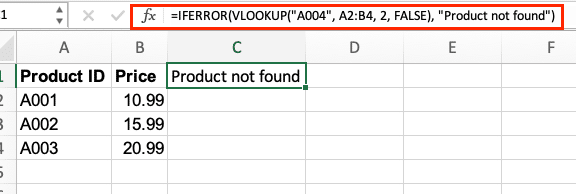
1. Example with specific values:

=IFERROR(VLOOKUP(“A004”, A2:B4, 2, FALSE), “Product not found”)

Returning Blank Cells Instead of Errors

Sometimes you want errors to appear as empty cells:

1. Use an empty string:

=IFERROR(YOUR_FORMULA, “”)

1. Common applications:

• Report generation
• Data import cleanup
• Lookup tables

Managing Multiple Error Conditions

For complex scenarios, nest IFERROR functions:

=IFERROR(Formula1,IFERROR(Formula2,”All attempts failed”))

Example with VLOOKUP:

=IFERROR(VLOOKUP(A1, Sheet1!A:B, 2, FALSE),IFERROR(VLOOKUP(A1, Sheet2!A:B, 2, FALSE),”Not found in any database”))

Working with Calculations and Zero Values

For financial calculations:

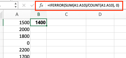
1. Convert errors to zero:

=IFERROR(SUM(A1:A10)/COUNT(A1:A10), 0)

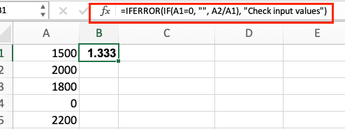
1. Handle multiple scenarios:

=IFERROR(IF(A1=0, “”, A2/A1), “Check input values”)

Next Steps

You’ve learned how to handle Excel errors effectively with IFERROR. From basic error handling to complex nested formulas, you can now create more reliable spreadsheets. For real-time data updates and automated report distribution, try Coefficient. It connects your spreadsheets directly to your business systems, ensuring your formulas always work with current data.

Get started with Coefficient today to automate your spreadsheet updates and maintain accurate calculations.