How to Extract Data from Excel Based on Criteria

Extracting specific data from large Excel spreadsheets can be a daunting task. Whether you’re an analyst crunching numbers or a manager preparing reports, knowing how to efficiently extract data based on criteria is crucial. This comprehensive guide will walk you through seven powerful methods to extract data from Excel, ranging from basic filters to advanced Power Query techniques.

Basic Methods for Extracting Data Based on Criteria

Using Excel’s Filter Function

Excel’s built-in filter function is a quick and user-friendly way to extract data based on specific criteria. This method is particularly useful for those new to Excel or for simple extraction tasks that don’t require complex formulas or advanced techniques.

Let’s use a sample dataset to demonstrate how to use the filter function effectively:

Order ID	Customer Name	Product	Quantity	Order Date	Total Value
1001	John Smith	Laptop	2	1/15/2024	$2,000
1002	Sarah Johnson	Smartphone	1	1/17/2024	$800
1003	Michael Brown	Tablet	3	1/20/2024	$1,500
1004	Emily Davis	Laptop	1	1/22/2024	$1,000
1005	David Wilson	Smartphone	2	1/25/2024	$1,600

To apply filters and extract data:

Step 1: Select your data range Click and drag to highlight your entire dataset, including the header row.

Step 2: Enable filters Navigate to the “Data” tab on the ribbon and click “Filter“. You should see small dropdown arrows appear in each column header.

Step 3: Apply your desired criteria Click the filter arrow in the column header you want to filter by. For example, to extract all laptop orders:

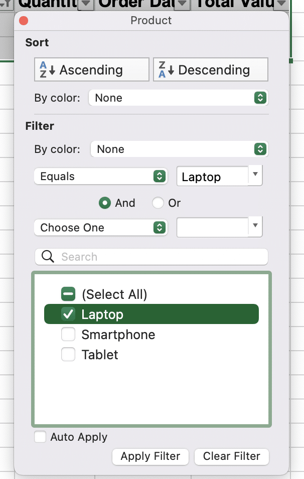
• Click the filter arrow in the “Product” column
• Uncheck “Select All“
• Check the box next to “Laptop“
• Click “Apply filter“

Step 4: Review your filtered data Your sheet will now display only the rows that meet your specified criteria.

For multiple criteria:

Step 1: Apply the first filter as described above

Step 2: Add additional filters to other columns as needed. For instance, to further filter laptop orders with a quantity greater than 1:

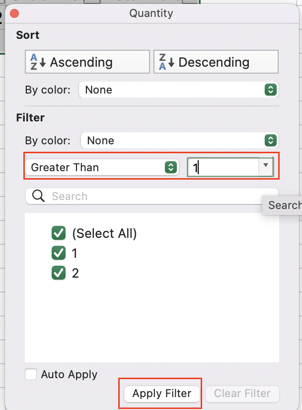
• Click the filter arrow in the “Quantity” column
• Select “Number Filters” > “Greater Than“
• Enter “1” in the dialog box and click “Apply fliter“

The filter function offers several advantages:

• Ease of use: It requires no formula knowledge and can be applied with just a few clicks.
• Visual feedback: You can quickly see the results of your filtering in real-time.
• Flexibility: Filters can be easily adjusted or removed as needed.

However, it also has some limitations:

• It doesn’t create a separate extracted dataset, which may be necessary for some analyses.
• Complex criteria can become cumbersome to manage with multiple filters.
• The original data order is maintained, which might not always be ideal for analysis.

Despite these limitations, the filter function remains a powerful tool for quick data extraction tasks and is an excellent starting point for users of all skill levels.

Sorting Data to Isolate Criteria

While not a direct extraction method, sorting is a fundamental technique that can help isolate data based on specific criteria. It’s often used in conjunction with other methods to organize data before extraction or to quickly identify patterns and outliers.

Using our previous dataset:

Order ID	Customer Name	Product	Quantity	Order Date	Total Value
1001	John Smith	Laptop	2	1/15/2024	$2,000
1002	Sarah Johnson	Smartphone	1	1/17/2024	$800
1003	Michael Brown	Tablet	3	1/20/2024	$1,500
1004	Emily Davis	Laptop	1	1/22/2024	$1,000
1005	David Wilson	Smartphone	2	1/25/2024	$1,600

To sort data:

Step 1: Select your data range. Click and drag to highlight your entire dataset, including the header row.

Step 2: Open the Sort dialog Navigate to the “Data” tab on the ribbon and click “Sort“.

Step 3: Choose your sort criteria In the Sort dialog box:

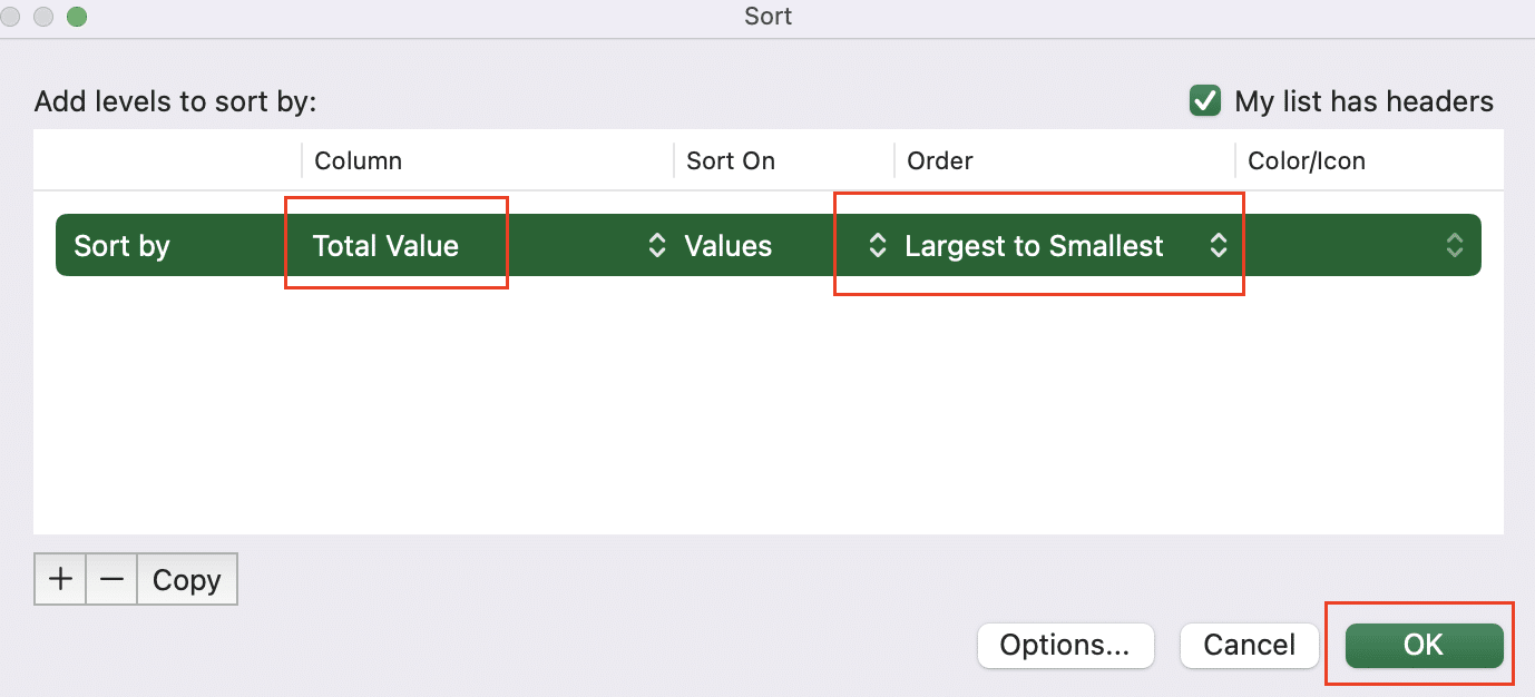
• Select the column you want to sort by (e.g., “Total Value”)
• Choose the sort order (Largest to Smallest for descending order)
• Click “OK“

Your data will now be sorted based on the specified criteria, with the highest value orders at the top.

For multiple sort levels:

Step 1: Open the Sort dialog as described above

Step 2: Add sort levels

• Click “Add Level” in the Sort dialog box

• Select an additional column to sort by (e.g., “Product”)

• Choose the sort order (A to Z for alphabetical order)
• Repeat for any additional sort criteria
• Click “OK“

This will sort your data first by Total Value, then by Product within each Total Value group.

While sorting is a powerful organizational tool, it has some limitations for data extraction:

• It alters the original order of your dataset, which may not always be desirable.
• It doesn’t actually extract or isolate data; it merely rearranges it.
• For complex criteria, sorting alone may not be sufficient to isolate the desired data.

Despite these limitations, sorting remains an essential skill in data analysis and is often used in combination with other extraction methods to achieve desired results.

Advanced Excel Functions for Data Extraction

VLOOKUP for Criteria-Based Extraction

VLOOKUP is a powerful function for extracting data based on a specific lookup value. It’s particularly useful when you need to pull information from one table into another based on a common identifier.

Let’s use an expanded version of our previous dataset to demonstrate VLOOKUP:

Table 1: Order Data

Order ID	Customer ID	Product	Quantity	Order Date	Total Value
1001	C001	Laptop	2	1/15/2024	$2,000
1002	C002	Smartphone	1	1/17/2024	$800
1003	C003	Tablet	3	1/20/2024	$1,500
1004	C004	Laptop	1	1/22/2024	$1,000
1005	C005	Smartphone	2	1/25/2024	$1,600

Table 2: Customer Data

Customer ID	Customer Name	Email	City
1001	John Smith	john@example.com	New York
1002	Sarah Johnson	sarah@example.com	Los Angeles
1003	Michael Brown	michael@example.com	Chicago
1004	Emily Davis	emily@example.com	Houston
1005	David Wilson	david@example.com	Phoenix

Now, let’s say we want to extract the customer’s email address based on the Order ID.

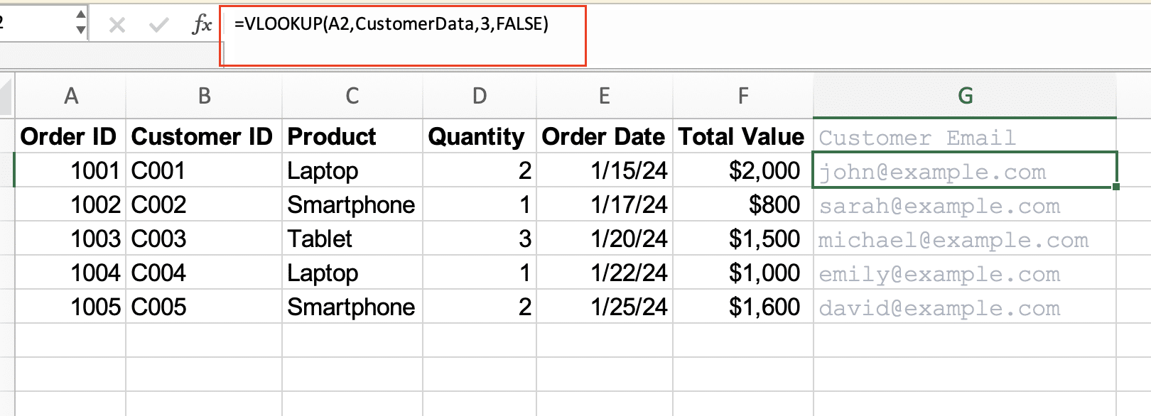
Step 1: Set up your VLOOKUP formula In a new cell, enter the following formula:

=VLOOKUP(A2, CustomerData, 3, FALSE)

Where:

• A2 contains the Customer ID from the Order Data table
• Customer Data is the named range containing your Customer Data table
• 3 is the column number in the Customer Data table containing email addresses
• FALSE specifies an exact match

Step 2: Apply the formula down to apply it to all orders.

Your result should look like this:

Order ID	Customer ID	Product	Quantity	Order Date	Total Value	Customer Email
1001	C001	Laptop	2	1/15/2024	$2,000	john@example.com
1002	C002	Smartphone	1	1/17/2024	$800	sarah@example.com
1003	C003	Tablet	3	1/20/2024	$1,500	michael@example.com
1004	C004	Laptop	1	1/22/2024	$1,000	emily@example.com
1005	C005	Smartphone	2	1/25/2024	$1,600	david@example.com

Tips for using VLOOKUP effectively:

• Ensure your lookup column (Customer ID in this case) is the leftmost column in the table array (CustomerData).
• Use FALSE for the range_lookup parameter to specify an exact match and avoid errors with sorted data.
• Wrap VLOOKUP in an IFERROR function to handle missing values:

=IFERROR(VLOOKUP(A2, CustomerData, 3, FALSE), “Not Found”)

This will display “Not Found” instead of an error if the Customer ID doesn’t exist in the Customer Data table.

VLOOKUP is an excellent tool for straightforward data extraction tasks, but it does have limitations. For more complex scenarios or when working with large datasets, you might want to consider the INDEX and MATCH combination or more advanced techniques.

INDEX and MATCH Combination

The INDEX and MATCH combination offers more flexibility than VLOOKUP, especially for large datasets or when lookup columns aren’t leftmost in the reference table. This method is particularly useful for two-way lookups and when you need to frequently change the column you’re extracting data from.

Using our previous dataset:

Table 1: Order Data

Order ID	Customer ID	Product	Quantity	Order Date	Total Value
1001	C001	Laptop	2	1/15/2024	$2,000
1002	C002	Smartphone	1	1/17/2024	$800
1003	C003	Tablet	3	1/20/2024	$1,500
1004	C004	Laptop	1	1/22/2024	$1,000
1005	C005	Smartphone	2	1/25/2024	$1,600

Table 2: Customer Data

Customer ID	Customer Name	Email	City
C001	John Smith	john@example.com	New York
C002	Sarah Johnson	sarah@example.com	Los Angeles
C003	Michael Brown	michael@example.com	Chicago
C004	Emily Davis	emily@example.com	Houston
C005	David Wilson	david@example.com	Phoenix

Let’s extract the customer’s city based on the Customer ID:

Step 1: Set up your INDEX-MATCH formula In a new cell, enter the following formula:

=INDEX(CustomerData[City], MATCH(B2, CustomerData[Customer ID], 0))

Where:

• CustomerData[City] is the column containing city names in the Customer Data table
• B2 contains the Customer ID from the Order Data table
• CustomerData[Customer ID] is the column of Customer IDs in the Customer Data table
• 0 specifies an exact match

Step 2: Apply the formula  the formula down to apply it to all orders.

Your result should look like this:

Order ID	Customer ID	Product	Quantity	Order Date	Total Value	Customer City
1001	C001	Laptop	2	1/15/2024	$2,000	New York
1002	C002	Smartphone	1	1/17/2024	$800	Los Angeles
1003	C003	Tablet	3	1/20/2024	$1,500	Chicago
1004	C004	Laptop	1	1/22/2024	$1,000	Houston
1005	C005	Smartphone	2	1/25/2024	$1,600	Phoenix

The INDEX-MATCH combination offers several advantages:

1. Flexibility: You can look up values in any column, not just the leftmost one.
2. Performance: It’s generally faster than VLOOKUP for large datasets.
3. Ease of modification: You can easily change the column you’re extracting from without rewriting the entire formula.

For multiple criteria lookups, you can use an array formula with INDEX-MATCH:

Step 1: Set up your multiple criteria INDEX-MATCH formula Enter the following formula (remember to press Ctrl+Shift+Enter to make it an array formula):

=INDEX(CustomerData[Email], MATCH(1, (CustomerData[Customer ID]=B2)*(CustomerData[City]=”New York”), 0))

This formula will return the email address for a customer with a specific ID who lives in New York.

Step 2: Apply the formula  the formula down to apply it to all relevant orders.

The INDEX-MATCH combination is a powerful tool for data extraction, offering more flexibility and efficiency than VLOOKUP in many scenarios. However, it can be more complex to write and understand, especially for Excel beginners. As you become more comfortable with these functions, you’ll find that they open up new possibilities for data analysis and extraction in Excel.

FILTER Function (for Excel 365 users)

The FILTER function, available in Excel 365, simplifies complex data extraction tasks by allowing you to specify multiple criteria directly within a single function. This dynamic array function returns all rows that meet the specified criteria, making it incredibly powerful for data extraction.

Let’s use our sample dataset to demonstrate the FILTER function:

Order ID	Customer ID	Product	Quantity	Order Date	Total Value
1001	C001	Laptop	2	1/15/2024	$2,000
1002	C002	Smartphone	1	1/17/2024	$800
1003	C003	Tablet	3	1/20/2024	$1,500
1004	C004	Laptop	1	1/22/2024	$1,000
1005	C005	Smartphone	2	1/25/2024	$1,600

To extract all orders for laptops with a quantity greater than 1:

Step 1: Set up your FILTER formula In a new cell, enter the following formula:

=FILTER(A2:F6, (C2:C6=”Laptop”)*(D2:D6>1))

Where:

• A2:F6 is the range containing your order data
• C2:C6=”Laptop” checks if the product is a laptop
• D2:D6>1 checks if the quantity is greater than 1

Step 2: Press Enter to apply the formula The FILTER function will automatically return all matching rows.

Your result should look like this:

Order ID	Customer ID	Product	Quantity	Order Date	Total Value
1001	C001	Laptop	2	1/15/2024	$2,000

The FILTER function offers several advantages:

1. Simplicity: It combines criteria specification and data extraction in a single function.
2. Dynamic output: The result automatically adjusts if the source data changes.
3. Multiple criteria: You can easily combine multiple conditions within one function.

You can also combine FILTER with other functions for more complex extractions:

Step 1: Set up a complex FILTER formula To extract all orders with a total value above the average:

=FILTER(A2:F6, F2:F6>AVERAGE(F2:F6))

Step 2: Press Enter to apply the formula

This will return all orders with a total value above the average of all orders.

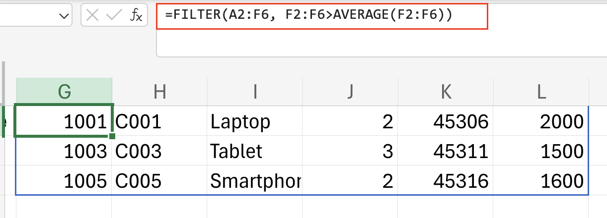
The FILTER function is a powerful tool for Excel 365 users, offering a streamlined approach to data extraction that can handle complex criteria with ease. While it’s not available in older versions of Excel, for those with access, it represents a significant advancement in Excel’s data manipulation capabilities.

Power Query: A Powerful Tool for Data Extraction

Introduction to Power Query

Power Query is a robust data transformation and extraction tool built into Excel. It provides a more visual and intuitive interface for complex data operations, making it easier to handle large datasets and perform advanced data manipulations.

Key benefits of Power Query include:

1. Efficiency: Handles large datasets more efficiently than traditional Excel functions.
2. Reproducibility: Creates step-by-step queries that can be easily modified or reapplied to updated data.
3. Data cleaning: Offers advanced options for cleaning and transforming data during the extraction process.
4. Multiple data sources: Can combine data from various sources, including other Excel sheets, CSV files, databases, and web pages.

To access Power Query:

Step 1: Open the Power Query Editor

• In Excel, click the “Data” tab on the ribbon

• Select “Get Data” > “From Table/Range” if your data is already in Excel, or choose the appropriate source if importing from elsewhere

Step 2: Select your data range If using data from your current Excel sheet, select the range containing your data (including headers).

Step 3: Load to Power Query Editor Click “OK” to load your selected data into the Power Query Editor.

You’ll now see the Power Query Editor interface, which provides a preview of your data and a series of transformation options.

Using Power Query for Criteria-Based Extraction

Let’s use our sample dataset to demonstrate how to extract data based on specific criteria using Power Query:

Order ID	Customer ID	Product	Quantity	Order Date	Total Value
1001	C001	Laptop	2	1/15/2024	$2,000
1002	C002	Smartphone	1	1/17/2024	$800
1003	C003	Tablet	3	1/20/2024	$1,500
1004	C004	Laptop	1	1/22/2024	$1,000
1005	C005	Smartphone	2	1/25/2024	$1,600

To extract all laptop orders with a total value greater than $1,500:

Step 1: Filter the Product column

• Click the dropdown arrow next to the “Product” column header
• Uncheck all boxes except “Laptop“

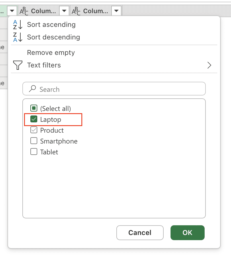
• Click “OK“

Step 2: Filter the Total Value column

• Click the dropdown arrow next to the “Total Value” column header
• Select “Number Filters” > “Greater Than“

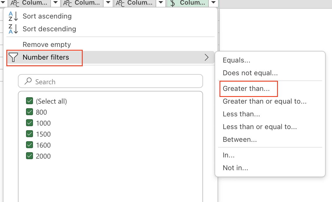
• Enter “1500” in the dialog box

• Click “OK“

Step 3: Review and refine your query

• Check the “Applied Steps” pane on the right to see a record of your actions

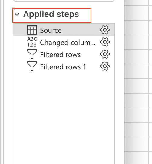
• Modify or remove steps as needed

Step 4: Load the extracted data

• Click “Close & Load” in the Home tab

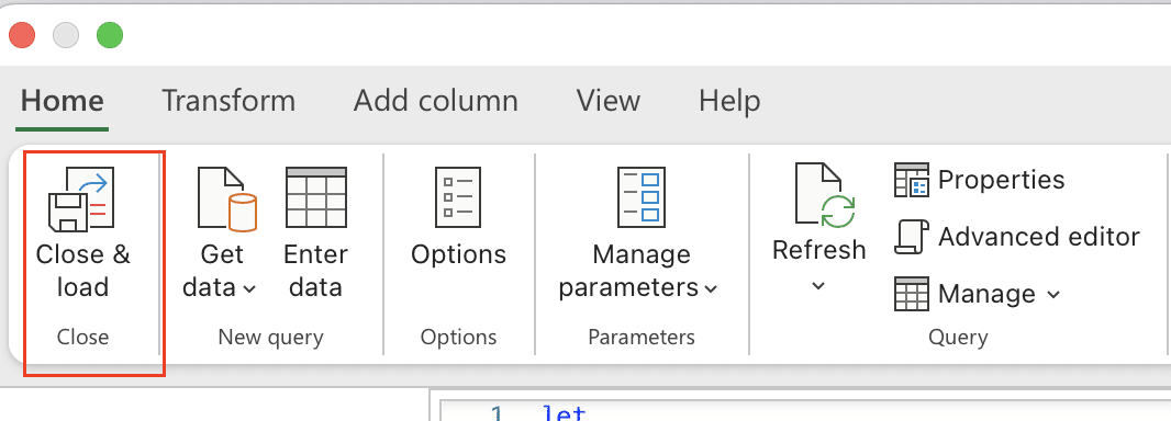
• Choose where to place the extracted data in your workbook

Your result will be a new table containing only the laptop orders with a total value greater than $1,500.

Power Query offers numerous advanced features for data extraction and transformation:

1. Merging queries: Combine data from multiple sources based on common columns.
2. Grouping: Aggregate data based on specific criteria.
3. Pivoting and unpivoting: Reshape your data for analysis.
4. Custom columns: Create new columns using Power Query’s M language for complex calculations.

For example, to group your data by product and calculate the total sales:

Step 1: Select the Product column Click on the “Product” column header to select it.

Step 2: Group by Product

• Go to the “Transform” tab

• Click “Group By“

• In the Group By dialog:
  • Group by: Product
  • New column name: Total Sales
  • Operation: Sum
  • Column: Total Value

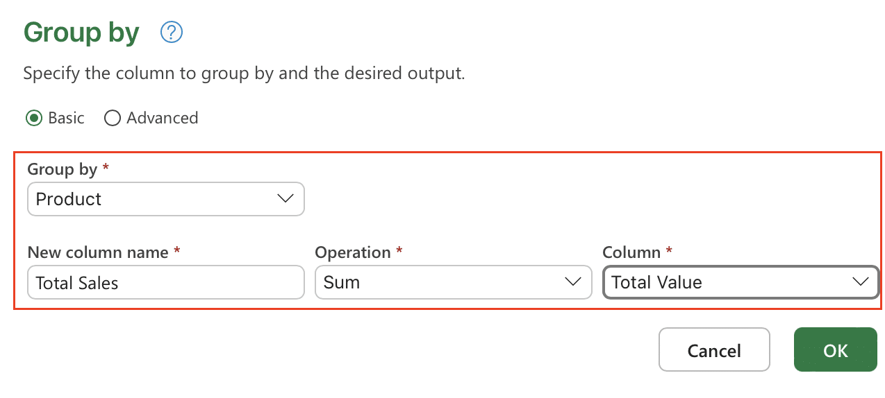
Step 3: Review and load Check your grouped data and click “Close & Load” when satisfied.

This will create a summary table showing total sales for each product type.

Power Query’s ability to handle complex data extraction and transformation tasks makes it an invaluable tool for data analysts and Excel power users. While it may have a steeper learning curve than some of the other methods we’ve discussed, its power and flexibility make it well worth the investment for those who frequently work with large or complex datasets.

Understanding Data Extraction in Excel

What is Data Extraction?

Data extraction in Excel is the process of retrieving specific information from a larger dataset based on defined criteria.  It enables analysts to:

• Isolate trends and patterns within subsets of data
• Generate targeted reports for specific departments or stakeholders
• Clean and organize information for further analysis or presentation

Common scenarios where data extraction proves invaluable include:

1. Sales teams filtering transaction data by region or date range to identify top-performing products
2. HR departments extracting employee information based on performance metrics or tenure
3. Inventory managers isolating stock items below reorder thresholds

By mastering data extraction techniques, you’ll not only save countless hours of manual data sorting but also significantly improve the accuracy of your reports. This skill empowers you to make data-driven decisions more efficiently, providing a competitive edge in today’s information-driven business landscape.

Preparing Your Excel Sheet for Data Extraction

Before diving into extraction methods, it’s crucial to organize your data properly. A well-structured dataset is the foundation for efficient and accurate data extraction. Follow these best practices to prepare your Excel sheet:

1. Structure your data in a tabular format: Ensure each column represents a single type of data and each row represents a unique record.
2. Use consistent formatting: Apply uniform formatting across columns, especially for date, currency, and numeric values.
3. Eliminate blank rows and columns: Remove any empty rows or columns that might interfere with data extraction processes.
4. Create a clear header row: Use descriptive, unique names for each column in the first row of your dataset.
5. Remove merged cells: Unmerge any merged cells, as they can complicate data extraction formulas and functions.

To optimize your data organization further, consider these additional tips:

• Use descriptive column headers: Opt for clear, concise names without spaces (e.g., “CustomerID” instead of “Customer ID”).
• Avoid special characters: Steer clear of symbols or special characters in cell values that might cause issues in formulas or filtering.
• Ensure data type consistency: Maintain uniform data types within each column (e.g., all dates in the same format, all numbers as values rather than text).

By implementing these practices, you’ll create a robust foundation for efficient data extraction, regardless of the method you choose to employ.

Automating Data Extraction in Excel

Using Coefficient for Seamless Data Extraction and Syncing

Coefficient is a powerful tool that simplifies data extraction and syncing between Excel and other applications. It’s particularly useful for teams that need to maintain up-to-date data across multiple platforms or for individuals who frequently pull data from various sources into Excel for analysis.

Key features of Coefficient include:

1. Real-time data syncing: Automatically update your Excel sheets with the latest data from connected sources.
2. Scheduled extractions: Set up regular data pulls without manual intervention.
3. Multiple data source integration: Connect to popular databases, CRMs, and other business tools.
4. No-code interface: Easily set up data connections and extractions without programming knowledge.

Learn how to set up Coefficient in Excel in the following video.

https://www.youtube.com/watch?v=sBg2goL8e_4

Creating Macros for Repeated Extractions

For users who prefer to stay within the Excel environment, macros offer a powerful way to automate repetitive data extraction tasks. By recording a series of actions and saving them as a macro, you can replay complex extraction processes with a single click.

Let’s create a simple macro to extract all orders for a specific product:

Step 1: Enable the Developer tab

• Go to File > Options > Customize Ribbon
• Check the box next to “Developer” under Main Tabs

Step 2: Start recording a macro

• Go to the Developer tab
• Click “Record Macro“
• Name your macro (e.g., “ExtractLaptopOrders”)

• Assign a shortcut key if desired
• Click “OK“

Step 3: Perform your extraction steps

• Select your data range
• Go to Data > Filter

• Click the filter dropdown for the Product column
• Select only “Laptop“

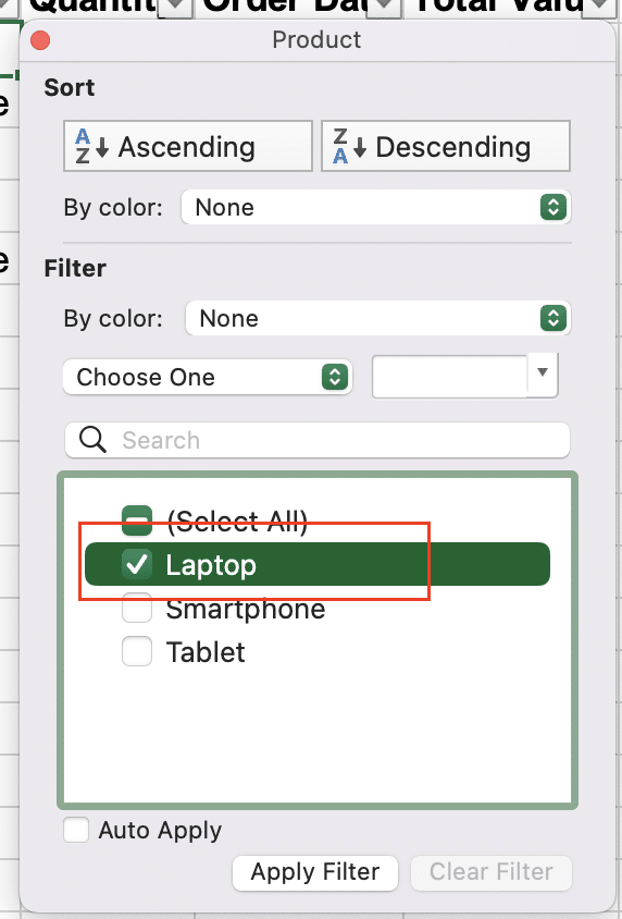
• Click “Apply Filter“

Step 4: Stop recording

• Go back to the Developer tab
• Click “Stop Recording“

Now you have a macro that will automatically filter your data to show only laptop orders. To run the macro:

• Use the assigned shortcut key, or
• Go to Developer > Macros, select your macro, and click “Run“

To edit your macro for more flexibility:

Step 1: Open the Visual Basic Editor

• Go to Developer > Visual Basic

Step 2: Locate your macro

• In the Project Explorer, find your workbook and expand Modules
• Double-click the module containing your macro

Step 3: Edit the VBA code You might modify the code to accept a product name as an input, making the macro more versatile:

vba

Sub ExtractProductOrders(productName As String)

    ActiveSheet.Range(“A1”).AutoFilter

    ActiveSheet.Range(“A1”).AutoFilter Field:=3, Criteria1:=productName

End Sub

This modified macro allows you to extract orders for any product by calling it with different product names.

Scheduling Automated Extractions

For truly hands-off data extraction, you can schedule your Excel macros to run automatically at set intervals.

To schedule automated extractions using Windows Task Scheduler:

Step 1: Save your Excel file with macros enabled Save your workbook as an .xlsm file.

Step 2: Create a batch file to run your Excel macro Create a new text file with the following content:

“C:Program FilesMicrosoft OfficerootOffice16EXCEL.EXE” “C:PathToYourWorkbook.xlsm” /r ExtractProductOrders

Save this file with a .bat extension.

Step 3: Set up a scheduled task

• Open Windows Task Scheduler
• Create a new task
• In the Actions tab, add a new action to start a program
• Browse to your batch file
• Set the trigger to your desired schedule (e.g., daily at 9 AM)

This setup will run your Excel macro automatically according to the schedule you’ve set, ensuring your data extractions are always up to date.

By leveraging these automation techniques, you can significantly reduce the time and effort required for regular data extractions, allowing you to focus more on analysis and decision-making based on the extracted data.

Master data extraction in Excel

Data extraction is just the beginning of the data analysis journey. By mastering these techniques, you’re equipping yourself with the tools to uncover valuable insights and make data-driven decisions more efficiently than ever before.

Ready to take your data extraction and syncing capabilities to the next level? Get started with Coefficient today and experience seamless, automated data workflows that will save you time and enhance your data analysis processes. With Coefficient, you can automate your data extraction tasks, ensure real-time data synchronization, and focus on deriving insights rather than managing data transfers.