How to Copy Data from One Sheet to Another in Excel

Want to transfer data between Excel sheets quickly and accurately? This guide covers five methods to copy information, from basic techniques to advanced automation.

Method 1: Quick Copy-Paste

The simplest way to copy data from one sheet to another in Excel is using the copy-paste function. Here’s how to do it:

Step 1. Select the data range in the source sheet.

• Click and drag your mouse to highlight the cells you want to copy.
• For non-contiguous selections, hold the Ctrl key while selecting multiple ranges.

Step 2. Copy the selected data.

• Press Ctrl+C on your keyboard.
• Alternatively, right-click the selected range and choose “Copy” from the context menu.

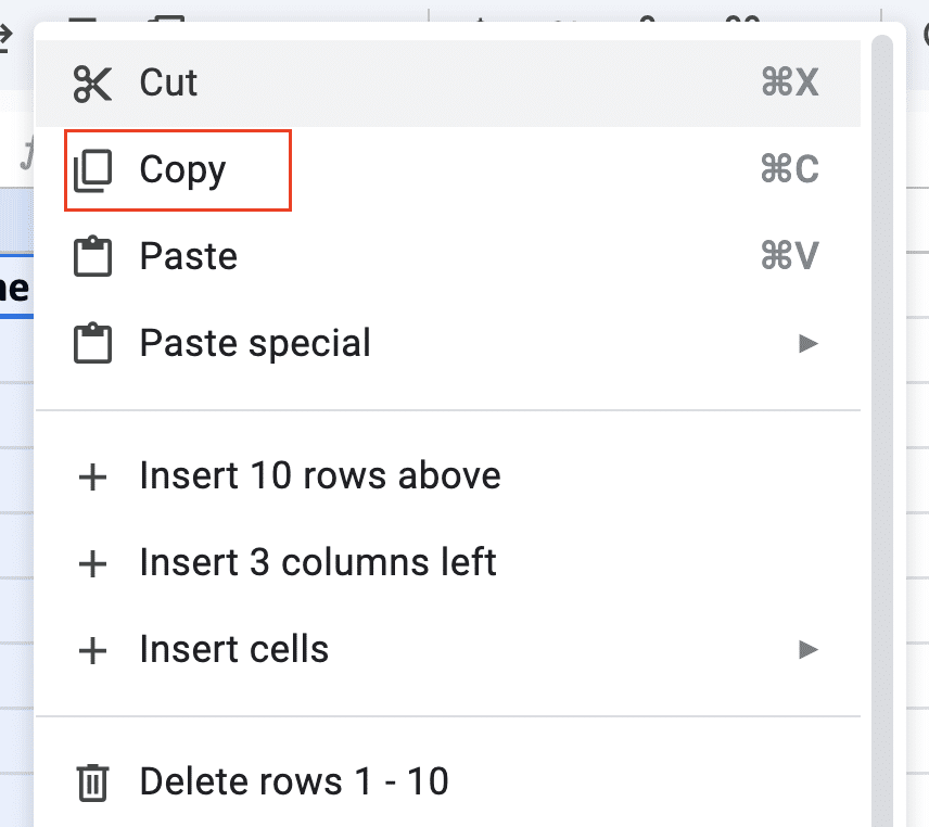
Step 3. Navigate to the destination sheet.

• Click the sheet tab at the bottom of the Excel window where you want to paste the data.
• If needed, create a new sheet by clicking the “+” icon next to the existing sheet tabs.

Step 4. Select the target cell in the destination sheet.

• Click on the cell where you want the top-left corner of your copied data to appear.

Step 5. Paste the data.

• Press Ctrl+V on your keyboard.
• Or right-click and select “Paste” from the context menu.

Tips for Preserving Formatting During Paste Operations

When copying data from one sheet to another in Excel, you may want to maintain specific formatting. Here are some tips:

1. Use “Paste Special” options:
   • After copying, right-click in the destination cell and select “Paste Special.”

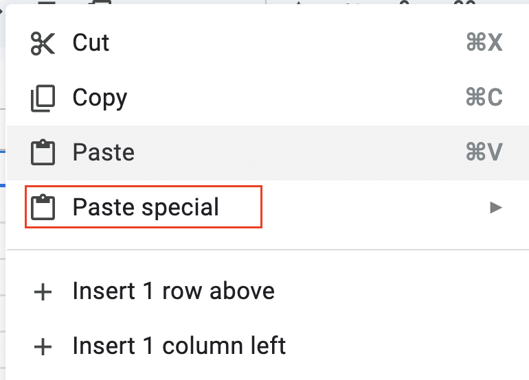
• Choose from options like “Values,” “Formats,” or “Formulas” to control what aspects of the copied data are transferred.

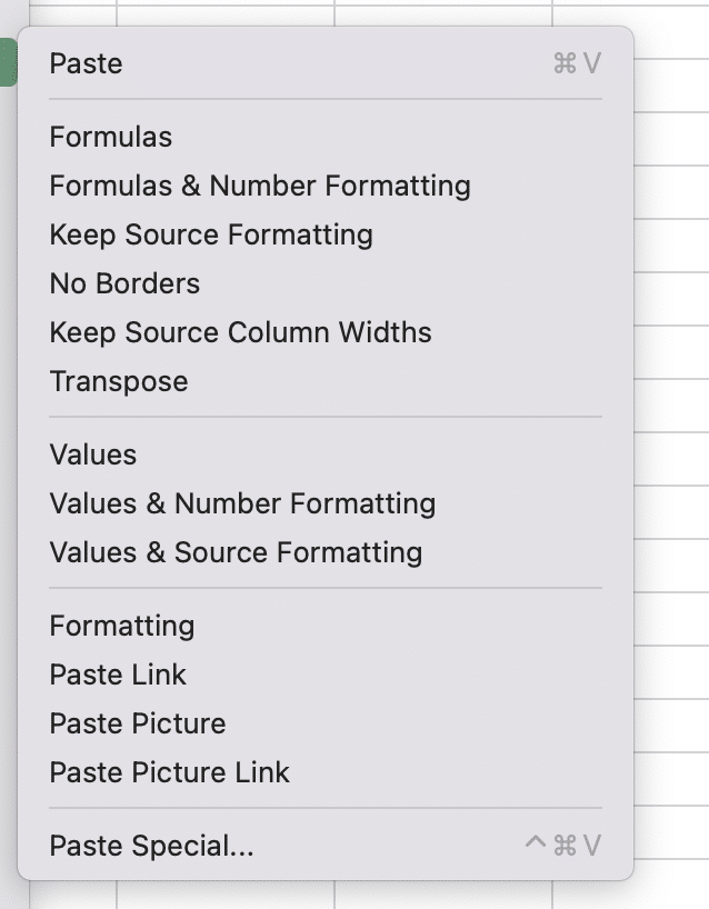
1. Keep Source Formatting:
   • Select “Keep Source Formatting” in the Paste Options to maintain the original look of your data.

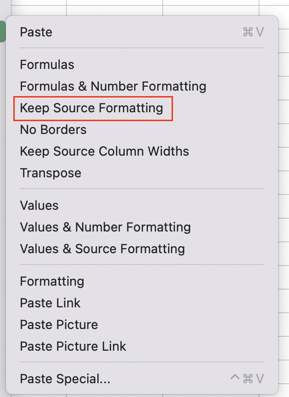
1. Use Paste Preview:
   • After pasting, the Paste Options button appears. Hover over different icons to preview how your data will look with various paste settings.

1. Keyboard Shortcuts:
   • Use Alt+E+S+V to paste values only, preserving the destination formatting.
   • Press Alt+E+S+T to paste the format only, without changing the existing values.

By mastering these copy-paste techniques, you can efficiently transfer data between Excel sheets while maintaining control over formatting.

Method 2: Using Formulas to Link Data Between Sheets

Basic Cell References

When you need to copy data from one sheet to another in Excel, using formulas with cell references provides a dynamic link. This method ensures that changes in the source sheet automatically update in the destination sheet.

Step 1. Understand the syntax for referencing cells in other sheets.

• The basic format is: =SheetName!CellReference
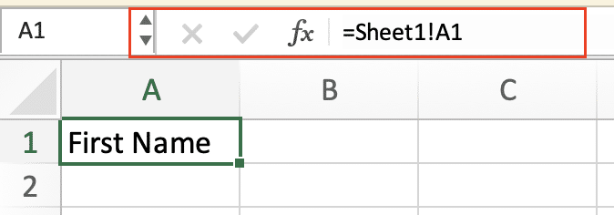
• For example, to reference cell A1 in Sheet1, use: =Sheet1!A1

Step 2. Reference a single cell from another sheet.

• In the destination sheet, select the cell where you want the data to appear.
• Type an equals sign (=) to start the formula.
• Enter the sheet name followed by an exclamation point (!), then the cell reference.
• Example: =Sheet1!A1

Step 3. Reference a range of cells across sheets.

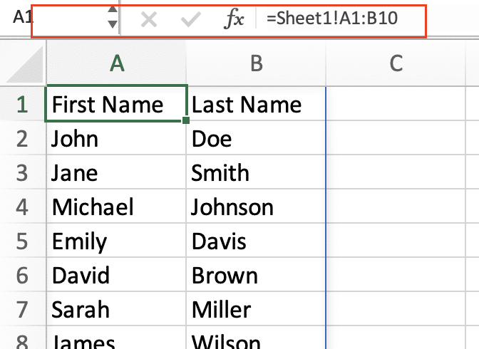
• Use the same syntax, but include the full range.
• Example: =Sheet1!A1:B10

Step 4. Handle sheet names with spaces or special characters.

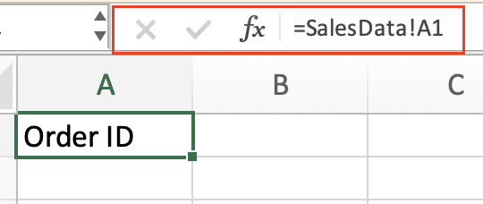
• Enclose the sheet name in single quotes.
• Example: =’Sales Data’!A1

Step 5. Copy the formula to additional cells as needed.

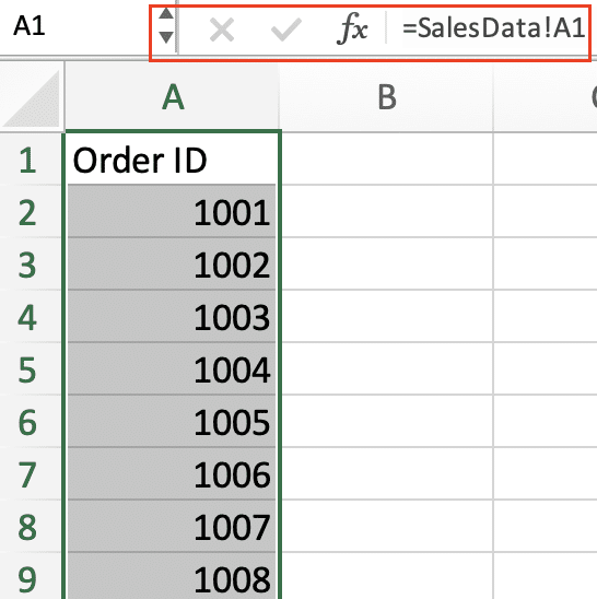
• Click and drag the fill handle (the small square in the bottom-right corner of the cell) to copy the formula to adjacent cells.

Tips for Using Cell References Across Sheets

1. Absolute vs. Relative References:
   • Use dollar signs ($) to create absolute references that don’t change when copied.
   • Example: =Sheet1!$A$1 will always refer to cell A1, even if the formula is copied.

1. Named Ranges:
   • Create named ranges in the source sheet for frequently used data.
   • Reference named ranges in formulas for cleaner, more readable formulas.
   • Example: =Sheet1!SalesData instead of =Sheet1!A1:B100

1. 3D References:
   • To reference the same cell or range across multiple sheets, use: =Sheet1:Sheet5!A1
   • This formula will sum the values in cell A1 from Sheet1 through Sheet5.

1. Error Handling:
   • Use the IFERROR function to manage potential errors when referencing other sheets.
   • Example: =IFERROR(Sheet1!A1, “Data not found”)

By mastering these techniques for using formulas to link data between sheets, you can create dynamic connections that update automatically, reducing manual data entry and potential errors.

Method 3: VLOOKUP for Automated Data Transfer

VLOOKUP is a powerful function for copying data from one sheet to another in Excel, especially when you need to match and retrieve information based on a common identifier.

VLOOKUP Function Syntax and Parameters

The VLOOKUP function has the following syntax: =VLOOKUP(lookup_value, table_array, col_index_num, [range_lookup])

• lookup_value: The value you want to find in the first column of the table_array.
• table_array: The range of cells containing the data you want to search through and retrieve.
• col_index_num: The column number in the table_array from which to retrieve the value.
• [range_lookup]: Optional. TRUE for approximate match (default), FALSE for exact match.

Setting Up the Source and Destination Sheets

Step 1. Organize your source data.

• Ensure your source data is in a tabular format with a unique identifier in the leftmost column.
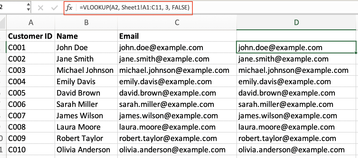
• Example: A customer database with Customer ID in column A, Name in B, and Email in C.

Step 2. Prepare your destination sheet.

• Create a column for the lookup value (e.g., Customer ID) in your destination sheet.
• Add columns for the data you want to retrieve (e.g., Name, Email).

Writing the VLOOKUP Formula for Data Copying

Step 3. Enter the VLOOKUP formula.

• In the destination sheet, select the cell where you want the retrieved data to appear.
• Type the VLOOKUP formula, referencing the source sheet.
• Example: =VLOOKUP(A2, Sheet1!A:C, 2, FALSE)

• A2 is the lookup value in the destination sheet.
• Sheet1!A:C is the table array in the source sheet.
• 2 indicates we want to retrieve data from the second column (Name).
• FALSE specifies an exact match.

Step 4. Copy the formula for multiple columns.

• Adjust the col_index_num to retrieve different columns.
• For Email: =VLOOKUP(A2, Sheet1!A:C, 3, FALSE)

Step 5. Extend the formula for multiple rows.

• Click and drag the fill handle to copy the formula down the column.

Advantages of Using VLOOKUP for Dynamic Updates

1. Automatic Updates: When source data changes, VLOOKUP formulas update automatically.
2. Flexibility: Easily modify the lookup criteria or retrieved columns without restructuring data.
3. Error Handling: Use IFERROR with VLOOKUP to manage missing data or errors gracefully.
4. Large Dataset Handling: VLOOKUP can efficiently handle large volumes of data.

Tips for Effective VLOOKUP Usage

1. Always use FALSE for the range_lookup parameter to ensure exact matches.
2. Combine VLOOKUP with INDEX and MATCH for more complex lookups.
3. Use named ranges to make formulas more readable and easier to maintain.
4. Consider using XLOOKUP (in newer Excel versions) for more versatile lookups.

By mastering VLOOKUP, you can automate data transfer between sheets, saving time and reducing errors in your Excel workflows.

Method 4: Copying Data with Excel’s Power Query

Power Query is a robust tool in Excel that allows you to import, transform, and load data from various sources, including other sheets within your workbook. Here’s how to use Power Query to copy data from one sheet to another in Excel:

Step 1. Access Power Query in Excel.

• In Excel 2016 and later: Go to the “Data” tab and click “Get Data” > “From Other Sources” > “From Table/Range.”

• In Excel 2013: Go to the “Power Query” tab and click “From Table.”

Step 2. Create a connection to the source sheet.

• Select the range of data in your source sheet you want to copy.
• Click “OK” to open the Power Query Editor.

Step 3. Select and transform data as needed.

• In the Power Query Editor, you can:
  • Remove or reorder columns
  • Filter rows
  • Change data types
  • Perform calculations

• Use the “Transform” tab to access various data manipulation options.

Step 4. Load the results to a new sheet.

• Once you’ve made your desired transformations, click “Close & Load” in the Home tab.
• In the “Import Data” dialog, choose “Table” and select “New worksheet.”
• Click “OK” to create a new sheet with your copied and transformed data.

Step 5. Refresh data to keep information up-to-date.

• To update the data in your destination sheet:
  • Right-click anywhere in the table and select “Refresh.”
  • Or go to the “Data” tab and click “Refresh All.”

Advantages of Using Power Query for Data Copying

1. Data Cleaning: Power Query offers powerful tools to clean and transform data during the copying process.
2. Automation: Once set up, you can refresh the data with a single click, automating regular updates.
3. Multiple Sources: Combine data from multiple sheets or even external sources in a single query.
4. Preserving Original Data: Power Query creates a separate copy, leaving your source data untouched.
5. Complex Transformations: Perform advanced operations like pivoting, unpivoting, and merging data sets.

Tips for Effective Power Query Usage

1. Use the “Applied Steps” pane to review and modify your data transformation process.
2. Save frequently used queries as functions for reuse across multiple workbooks.
3. Leverage Power Query’s M language for custom transformations beyond the built-in options.
4. Use “Parameters” to create flexible queries that can adapt to changing data ranges or criteria.

By mastering Power Query, you can efficiently copy and transform data between Excel sheets, handling complex data manipulation tasks with ease.

Method 5: VBA Macros for Automated Data Transfer

Visual Basic for Applications (VBA) macros provide a powerful way to automate data copying between sheets in Excel. Here’s how to create and use a VBA macro for this purpose:

Step 1. Open the Visual Basic Editor.

• Press Alt + F11 on your keyboard, or
• Go to the “Developer” tab and click “Visual Basic.”

Step 2. Insert a new module.

• In the VBA Editor, go to Insert > Module.

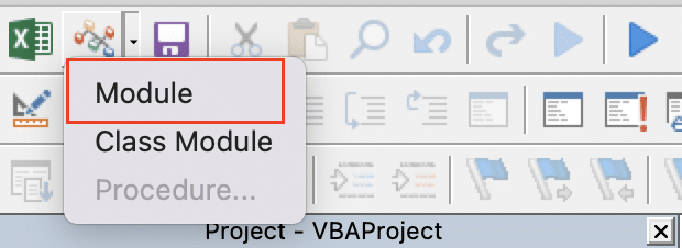
Step 3. Write a simple VBA script to copy data.

• In the new module, paste the following code:

vba

Copy

Sub CopyDataBetweenSheets()

    ‘ Define variables

    Dim sourceSheet As Worksheet

    Dim destinationSheet As Worksheet

    Dim lastRow As Long

    Dim lastColumn As Long

    ‘ Set source and destination sheets

    Set sourceSheet = ThisWorkbook.Sheets(“Sheet1”)

    Set destinationSheet = ThisWorkbook.Sheets(“Sheet2”)

    ‘ Find the last used row and column in the source sheet

    lastRow = sourceSheet.Cells(sourceSheet.Rows.Count, “A”).End(xlUp).Row

    lastColumn = sourceSheet.Cells(1, sourceSheet.Columns.Count).End(xlToLeft).Column

    ‘ Copy the data

    sourceSheet.Range(sourceSheet.Cells(1, 1), sourceSheet.Cells(lastRow, lastColumn)).Copy _

        Destination:=destinationSheet.Range(“A1”)

    ‘ Clean up

    Application.CutCopyMode = False

    MsgBox “Data copied successfully!”, vbInformation

End Sub

Step 4. Customize the script for specific needs.

• Modify the sheet names in the code to match your workbook.
• Adjust the range if you need to copy specific columns or rows.

Step 5. Run the macro manually.

• Return to your Excel workbook.
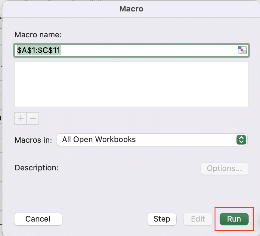
• Go to the “Developer” tab and click “Macros.”

• Select your macro and click “Run.”

Step 6. (Optional) Create a button to run the macro.

• Go to the “Developer” tab and click “Insert.”
• Choose a button shape and draw it on your worksheet.
• Assign the macro to the button when prompted.

Customizing the VBA Script

1. Conditional Copying: Add an If statement to copy only certain rows based on a condition:

vba

Copy

For i = 1 To lastRow

    If sourceSheet.Cells(i, 1).Value > 100 Then

        sourceSheet.Rows(i).Copy Destination:=destinationSheet.Rows(destinationSheet.Rows.Count).End(xlUp).Offset(1)

    End If

Next i

1. Error Handling: Implement error handling to make your macro more robust:

vba

Copy

On Error GoTo ErrorHandler

‘ Your existing code here

Exit Sub

ErrorHandler:

    MsgBox “An error occurred: ” & Err.Description, vbCritical

    Exit Sub

Considerations for Using Macros in Shared Workbooks

1. Security: Macros can pose security risks. Only run macros from trusted sources.
2. Compatibility: Ensure all users have macros enabled and the necessary permissions.
3. Version Control: Use comments in your VBA code to track changes and versions.
4. Performance: For large data sets, consider using arrays to improve speed.
5. Debugging: Use the VBA Editor’s debugging tools to step through your code and identify issues.

By leveraging VBA macros, you can create powerful, customized solutions for copying data between Excel sheets, automating complex tasks and saving significant time in your data management processes.

Method 6: Linking Workbooks for External Data Copying

When you need to copy data from one Excel workbook to another, creating external references provides a dynamic link between the files. This method ensures that changes in the source workbook automatically update in the destination workbook.

Creating External References Between Workbooks

Step 1. Open both the source and destination workbooks.

• Ensure both workbooks are open in Excel.

Step 2. In the destination workbook, select the cell where you want the data to appear.

Step 3. Type an equals sign (=) to start the formula.

Step 4. Switch to the source workbook and click the cell containing the data you want to reference.

• Excel will automatically create the correct syntax for the external reference.

Step 5. Press Enter to complete the formula.

Syntax for Referencing Cells in Other Workbooks

The general syntax for external references is: ='[Workbook Name]Sheet Name’!CellReference

For example: ='[Sales Data.xlsx]Sheet1′!A1

If the workbook name contains spaces, enclose it in single quotes: ='[Q3 Sales Data.xlsx]Sheet1′!A1

Managing Broken Links When Workbooks Are Moved

1. Use relative file paths:
   • If both workbooks are in the same folder, you can use a relative path.
   • Example: ='[Sales Data.xlsx]Sheet1′!A1

1. Update links manually:
   • Go to Data > Edit Links
   • Select the broken link and click “Change Source“
   • Navigate to the new location of the source workbook

1. Use the INDIRECT function for flexible references:
   • =INDIRECT(“‘[” & A1 & “]Sheet1’!A1”)
   • Where A1 contains the workbook name

Updating External References Automatically

1. Enable automatic updating:
   • Go to File > Options > Advanced
   • Under “When calculating this workbook” select “Update remote references”

1. Manual update:
   • Go to Data > Edit Links
   • Click “Update Values“

1. Use VBA to update links on workbook open:

vba

Copy

Private Sub Workbook_Open()

    ThisWorkbook.UpdateLink Name:=ThisWorkbook.LinkSources

End Sub

Tips for Effective External Referencing

1. Use named ranges in the source workbook for easier referencing and maintenance.
2. Consider using Power Query to import data from external workbooks for more complex scenarios.
3. Be cautious with circular references when linking workbooks bidirectionally.
4. Regularly check and update links to ensure data integrity.

By mastering external references, you can efficiently copy and link data between Excel workbooks, creating dynamic connections that update automatically and reduce manual data entry.

Wrapping Up: Choosing the Right Method

Select the most suitable data copying technique based on your specific needs, data volume, and desired level of automation. Experiment with different methods to optimize your Excel workflow and improve your data management efficiency.

Ready to take your Excel data management to the next level? Get started with Coefficient for advanced data integration and automation.