VLOOKUP allows you to compare data between two Excel sheets efficiently. This guide explains the process, from identifying common fields to interpreting results.

Comparing Two Excel Sheets with VLOOKUP: Step-by-Step Tutorial

Identify the Common Field Between Sheets

Selecting the right column for comparison is crucial when using VLOOKUP to compare two Excel sheets.

Step 1: Choose a unique identifier.

• Examine both sheets to find a column that contains unique values for each row.
• Common identifiers include employee IDs, product codes, or transaction numbers.
• Ensure this identifier is present in both sheets you want to compare.

Step 2: Verify data consistency.

• Check that the chosen identifier is formatted consistently across both sheets.
• Look for discrepancies like leading zeros, extra spaces, or capitalization differences.
• Use Excel’s data cleaning features to standardize the data if necessary.

Step 3: Position the identifier column.

• In the sheet where you’ll perform the VLOOKUP, place the identifier column on the left.
• VLOOKUP searches from left to right, so this positioning is essential for the function to work correctly.

Set Up Your VLOOKUP Formula

Understanding the VLOOKUP syntax is key to effectively comparing two Excel sheets.

Step 1: Open the VLOOKUP function.

• Click on the cell where you want the comparison result to appear.
• Type “=VLOOKUP(” to begin the formula.

Step 2: Enter the lookup value.

• This is the value you’re searching for in the second sheet.
• Usually, it’s a cell reference to your identifier in the current sheet.
• Example: A2 (if your identifier is in column A)

Step 3: Specify the table array.

• This is the range of cells in the second sheet that contains your data.
• Use an absolute reference to keep the range fixed when copying the formula.
• Example: Sheet2!$A$2:$D$100 (for a range from A2 to D100 in Sheet2)

Step 4: Indicate the column index number.

• This is the column number (counting from left) in your table array that contains the value you want to return.
• Example: 3 (if you want to return a value from the third column of your table array)

Step 5: Set the range lookup parameter.

• Use FALSE for an exact match or TRUE for an approximate match.
• For comparing sheets, you typically want an exact match, so use FALSE.

Step 6: Close the formula.

• Add a closing parenthesis and press Enter.

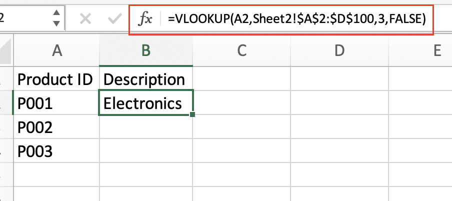
Your complete VLOOKUP formula should look similar to this: =VLOOKUP(A2,Sheet2!$A$2:$D$100,3,FALSE)

Apply VLOOKUP to Compare Sheets

Now that you’ve set up the VLOOKUP formula, it’s time to apply it to compare your Excel sheets.

Step 1: Enter the formula in the first cell.

• Click on the cell where you want your comparison results to start.
• Type or paste your VLOOKUP formula.
• Press Enter to see the result for the first row.

Step 2: Copy the formula to additional rows.

• Click on the cell with your VLOOKUP formula.
• Look for the small square in the bottom-right corner of the cell (the fill handle).
• Click and drag this handle down to copy the formula to as many rows as needed.

Step 3: Interpret the results.

• If VLOOKUP finds a match, it will return the value from the specified column in the second sheet.
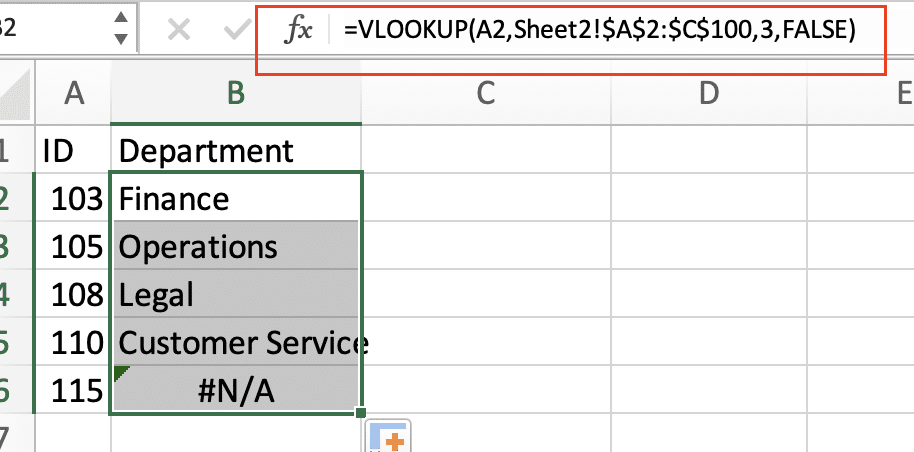
• If no match is found, you’ll see a #N/A error.

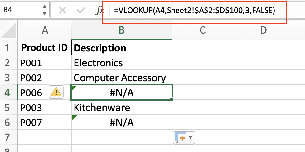
• Review these results to identify matches and discrepancies between your sheets.

Step 4: Handle errors (optional).

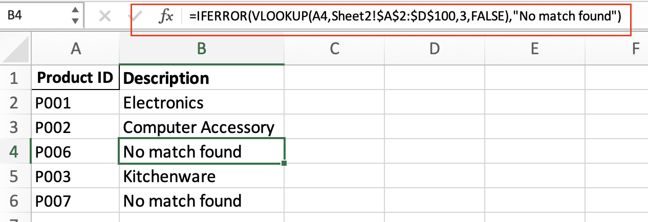
• To make your results cleaner, wrap your VLOOKUP in an IFERROR function.
• This allows you to display a custom message when no match is found.
• Example: =IFERROR(VLOOKUP(A2,Sheet2!$A$2:$D$100,3,FALSE),”No match found”)

How do I create a VLOOKUP between two sheets in Excel?

Creating a VLOOKUP between two sheets involves referencing data from one sheet while performing the lookup in another. Here’s a detailed breakdown of the process:

Step 1: Prepare your data.

• Ensure both sheets have a common identifier column.
• Organize your data so that the lookup column is on the left in the sheet you’re referencing.

Step 2: Start your VLOOKUP formula.

• In the sheet where you want the results, begin with =VLOOKUP(

Step 3: Enter the lookup value.

• This is typically a cell reference in your current sheet.
• Example: A2 (if your identifier is in column A)

Step 4: Specify the table array from the other sheet.

• Use the sheet name followed by an exclamation point, then the cell range.
• Make this reference absolute by adding dollar signs.
• Example: Sheet2!$A$2:$C$10

Step 5: Indicate the column index number.

• Count the columns in your table array, starting from the left.
• Enter the number of the column containing the data you want to return.
• Example: 3 (if you want data from the third column of your table array)

Step 6: Set the range lookup to FALSE for exact matches.

• This ensures VLOOKUP only returns exact matches.

Step 7: Close your formula and press Enter.

Your complete formula should look like this: =VLOOKUP(A2,Sheet2!$A$2:$C$10,3,FALSE)

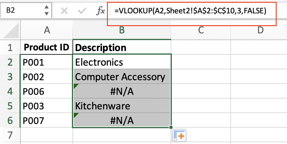
This formula looks up the value in A2 of the current sheet within the range A2:C10 of Sheet2, returning the value from the third column if an exact match is found.

Can you use VLOOKUP to compare two spreadsheets?

Yes, VLOOKUP is an excellent tool for comparing data between two spreadsheets. Here’s how to effectively use it for this purpose:

Step 1: Set up your comparison sheet.

• Create a new sheet or use an existing one for your comparison results.
• Copy the identifier column from one of your original sheets to this new sheet.

Step 2: Create column headers for your comparison.

• Label columns for data from both sheets and a column for the comparison result.
• Example headers: “ID”, “Sheet1 Data”, “Sheet2 Data”, “Match?”

Step 3: Use VLOOKUP to pull data from both sheets.

• In the “Sheet1 Data” column, use VLOOKUP to fetch data from the first sheet.
• In the “Sheet2 Data” column, use another VLOOKUP to fetch data from the second sheet.

Step 4: Compare the results.

• In the “Match?” column, use an IF statement to compare the two VLOOKUP results.
• Example formula: =IF(B2=C2,”Match”,”Mismatch”)

Step 5: Apply error handling.

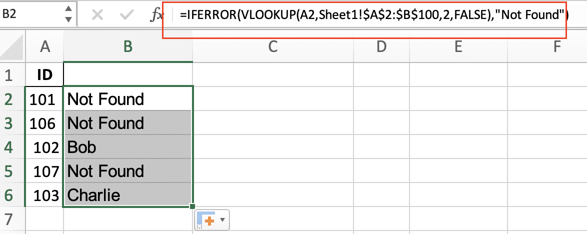
• Wrap your VLOOKUPs in IFERROR functions to handle cases where data isn’t found.
• Example: =IFERROR(VLOOKUP(A2,Sheet1!$A$2:$B$100,2,FALSE),”Not Found”)

Step 6: Analyze your results.

• Use Excel’s filtering and sorting features to identify matches and mismatches.
• Consider using conditional formatting to highlight discrepancies visually.

By following these steps, you can effectively use VLOOKUP to compare data across two spreadsheets, identifying matches and discrepancies with ease.

Enhancing Your VLOOKUP Comparisons

How do I compare two Excel spreadsheets for matching data?

Comparing two Excel spreadsheets for matching data involves more than just using VLOOKUP. Here’s a comprehensive approach:

Step 1: Prepare your data.

• Ensure both spreadsheets have a common identifier column.
• Clean and standardize your data to avoid false mismatches.

Step 2: Set up a comparison sheet.

• Create a new sheet for your comparison results.
• Copy the identifier column from one of your original sheets to this new sheet.

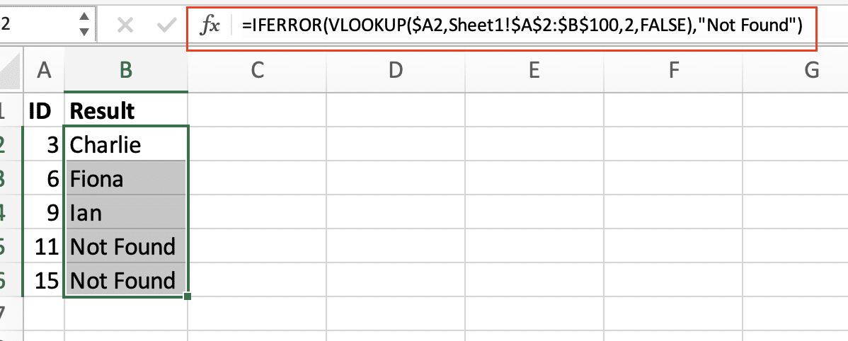
Step 3: Use VLOOKUP to pull data from both sheets.

• Create columns for data from both sheets.
• Use VLOOKUP to fetch corresponding data from each sheet.

Example formulas: Sheet1 Data: =IFERROR(VLOOKUP($A2,Sheet1!$A$2:$B$100,2,FALSE),”Not Found”)

Sheet2 Data: =IFERROR(VLOOKUP($A2,Sheet2!$A$2:$B$100,2,FALSE),”Not Found”)

Step 4: Create a comparison column.

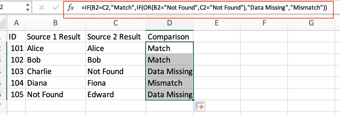
• Use an IF statement to compare the results from both VLOOKUPs.
• Example formula: =IF(B2=C2,”Match”,IF(OR(B2=”Not Found”,C2=”Not Found”),”Data Missing”,”Mismatch”))

Step 5: Summarize your results.

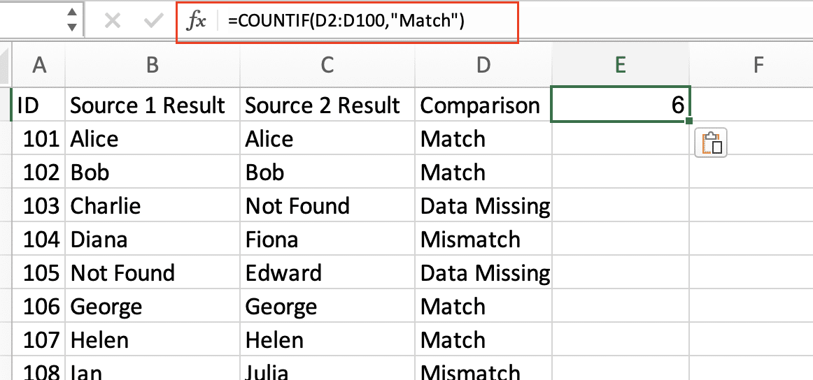
• Use COUNTIF functions to count matches, mismatches, and missing data.
• Example: =COUNTIF(D2:D100,”Match”)

Step 6: Visualize your comparison.

• Apply conditional formatting to highlight matches, mismatches, and missing data.
• Create a pie chart or bar graph to represent the proportion of matches vs. mismatches.

Step 7: Analyze discrepancies.

• Sort or filter your comparison sheet to focus on mismatches and missing data.
• Investigate these discrepancies to understand why the data doesn’t match.

By following these steps, you can create a comprehensive comparison of two Excel spreadsheets, identifying matching data, mismatches, and missing information.

How do I use VLOOKUP to find matches from another sheet?

VLOOKUP is an excellent tool for finding matches between sheets. Here’s how to use it effectively:

Step 1: Identify your lookup value.

• This is the value you’re searching for in the other sheet.
• It’s typically in a cell in your current sheet.

Step 2: Determine your table array.

• This is the range in the other sheet where you’re looking for matches.
• It must include the column with your lookup values and the column with the data you want to return.

Step 3: Count the column index number.

• This is the number of the column (counting from left) in your table array that contains the data you want to return.

Step 4: Decide on exact or approximate matching.

• Use FALSE for exact matches or TRUE for approximate matches.
• For finding specific matches between sheets, you typically want FALSE.

Step 5: Construct your VLOOKUP formula.

• Combine all these elements into your VLOOKUP formula.
• Example: =VLOOKUP(A2,Sheet2!$A$2:$C$100,3,FALSE)

Step 6: Apply error handling.

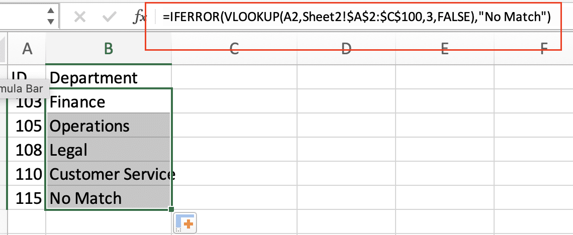
• Wrap your VLOOKUP in an IFERROR function to handle cases where no match is found.
• Example: =IFERROR(VLOOKUP(A2,Sheet2!$A$2:$C$100,3,FALSE),”No Match”)

Step 7: Copy the formula.

• Drag the formula down to apply it to all relevant rows.

Step 8: Analyze your results.

• Review the returned values to identify matches between your sheets.
• Use Excel’s filtering and sorting features to focus on specific results.

By following these steps, you can effectively use VLOOKUP to find matches from another sheet, making data comparison and analysis more efficient.

VLOOKUP Alternatives for Sheet Comparison

While VLOOKUP is a powerful tool for comparing sheets, Excel offers other functions that can be more flexible or efficient in certain situations:

XLOOKUP (for Excel 2021 and Microsoft 365)

XLOOKUP is a more versatile and user-friendly alternative to VLOOKUP.

Advantages:

• Can look both left and right
• Returns an exact match by default
• Can return multiple columns

Example syntax: =XLOOKUP(lookup_value, lookup_array, return_array, [if_not_found], [match_mode], [search_mode])

INDEX-MATCH Combination

This combination allows for more flexibility than VLOOKUP, especially for two-way lookups.

Advantages:

• Can look up values in any column, not just the leftmost
• More efficient for large datasets
• Can perform two-way lookups

Example syntax: =INDEX(return_range, MATCH(lookup_value, lookup_range, 0))

Power Query

For more complex sheet comparisons, Power Query offers advanced data manipulation capabilities.

Advantages:

• Can handle large datasets efficiently
• Allows for complex transformations and merges
• Creates a repeatable process for regular comparisons

To use Power Query:

1. Go to the Data tab
2. Click “Get Data” > “From Other Sources” > “Blank Query“

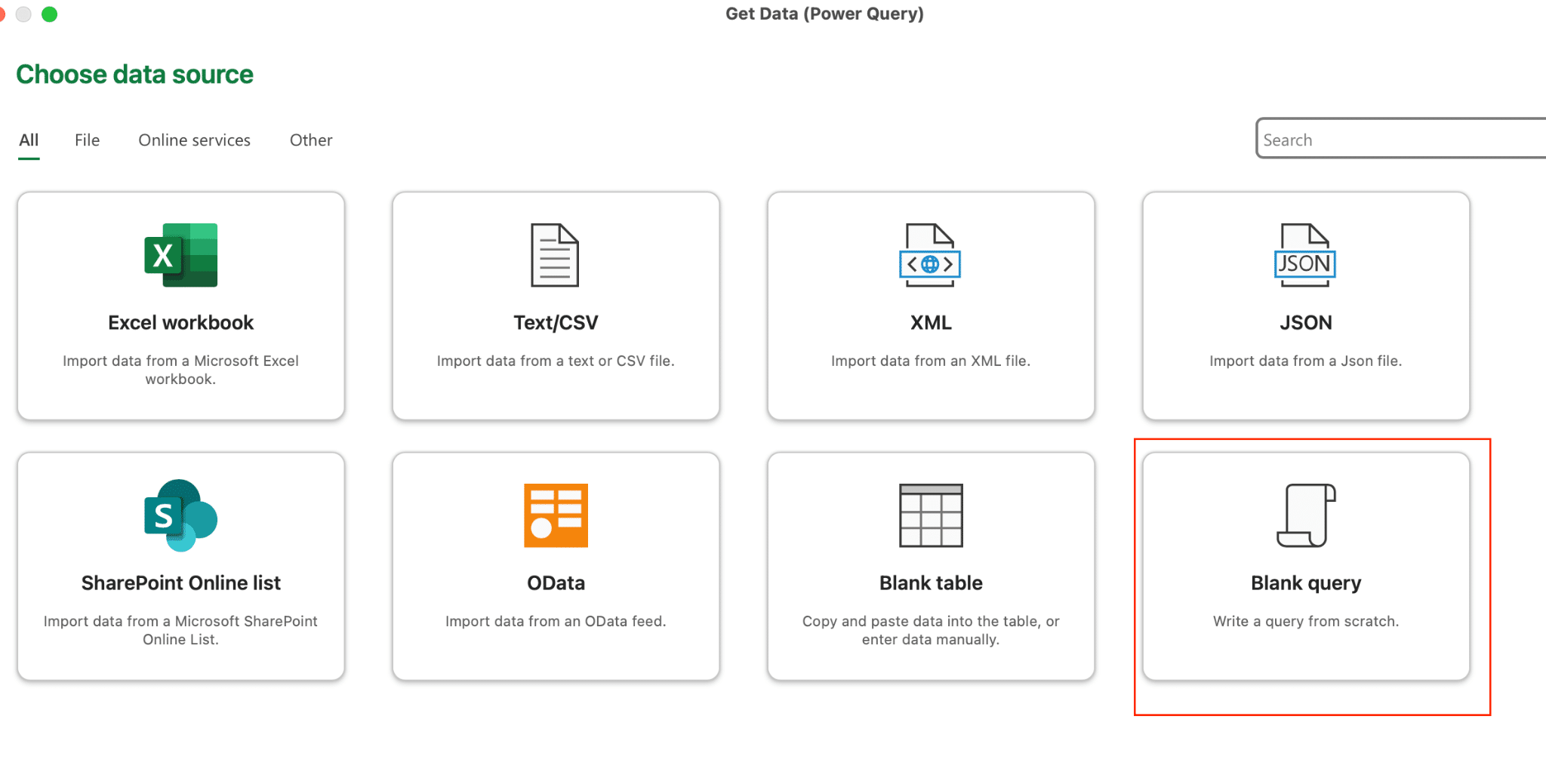
1. Use the Power Query Editor to import and manipulate your data

Wrap-up: Mastering Excel Sheet Comparisons

Comparing Excel sheets with VLOOKUP enhances data analysis efficiency. Practice these techniques to become proficient in identifying matches, discrepancies, and trends across multiple datasets.

Ready to take your Excel data analysis to the next level? Get started with Coefficient to seamlessly sync and compare data from various sources directly in your spreadsheets. Start your journey with Coefficient today and transform how you work with Excel data.