Working with horizontal data tables in Excel can be challenging, especially when you need to find specific information across rows. The HLOOKUP function solves this problem by letting you search horizontally arranged data efficiently. In this comprehensive guide, you’ll learn how to use HLOOKUP to retrieve data accurately and automate your lookup processes.

How to Use HLOOKUP in Excel

The HLOOKUP function follows a straightforward syntax but requires careful setup to work correctly. Let’s break down the basic formula structure:

=HLOOKUP(lookup_value, table_array, row_index_num, [range_lookup])

Where:

• lookup_value: The value you want to find in the first row
• table_array: The range containing your data
• row_index_num: The row number from which to retrieve the result
• range_lookup: TRUE for approximate match, FALSE for exact match (optional)

Creating Your First HLOOKUP Formula

Let’s start with a simple example using product data:

Product ID	Product A	Product B	Product C	Product D
Price	$10.99	$15.99	$20.99	$25.99
Stock	100	150	200	250

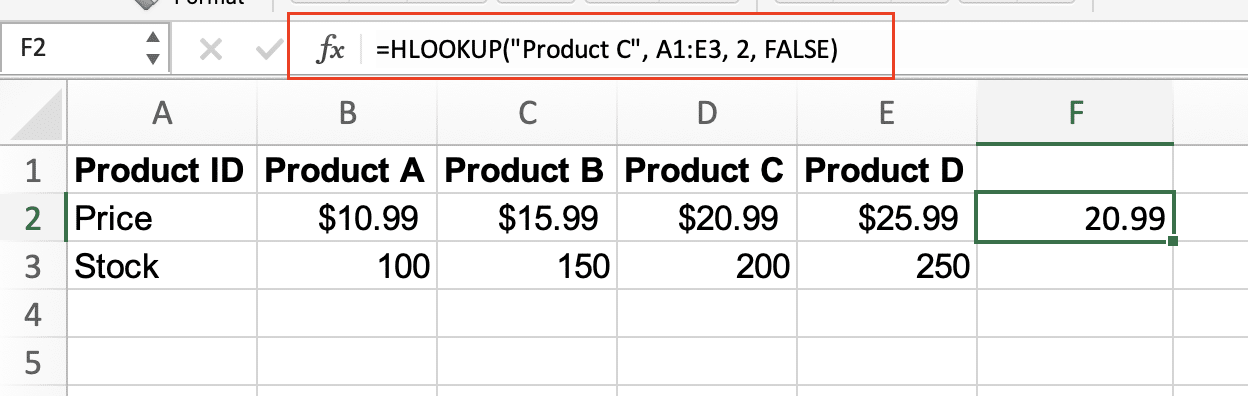
To find the price of Product C:

=HLOOKUP(“Product C”, A1:E3, 2, FALSE)

This returns: $20.99

To find the stock quantity of Product B:

=HLOOKUP(“Product B”, A1:E3, 3, FALSE)

This returns: 150

Key tips to prevent errors:

1. Ensure your lookup value exists in the first row
2. Count rows carefully when specifying row_index_num
3. Use FALSE for exact matches when working with text

Finding Exact Matches with HLOOKUP

When working with specific values, always use FALSE for the range_lookup parameter. Here’s a more complex example:

Code	ABC123	DEF456	GHI789	JKL012
Category	Tools	Parts	Supplies	Equipment
Supplier	Smith Co	Jones LLC	Brown Inc	Green Ltd

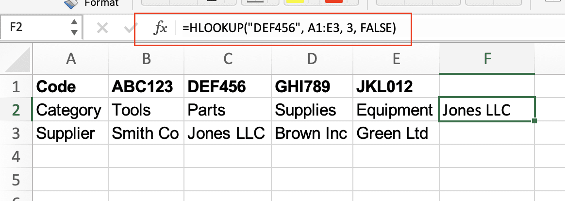
To find the supplier for code DEF456:

=HLOOKUP(“DEF456”, A1:E3, 3, FALSE)

This returns: Jones LLC

What’s the Difference Between VLOOKUP and HLOOKUP?

Understanding when to use HLOOKUP versus VLOOKUP is crucial:

Feature	HLOOKUP	VLOOKUP
Data Structure	Horizontal	Vertical
Search Direction	Top to bottom	Left to right
Best Use Case	Wide, short tables	Tall, narrow tables

Combining HLOOKUP with MATCH

The MATCH function can make HLOOKUP more dynamic by automatically determining the row number:

Region	North	South	East	West
Q1 Sales	10000	15000 Try the Free Spreadsheet Extension Over 500,000 Pros Are Raving About Stop exporting data manually. Sync data from your business systems into Google Sheets or Excel with Coefficient and set it on a refresh schedule. Get Started	12000	18000
Q2 Sales	12000	16000	13000	19000
Q3 Sales	13000	17000	14000	20000

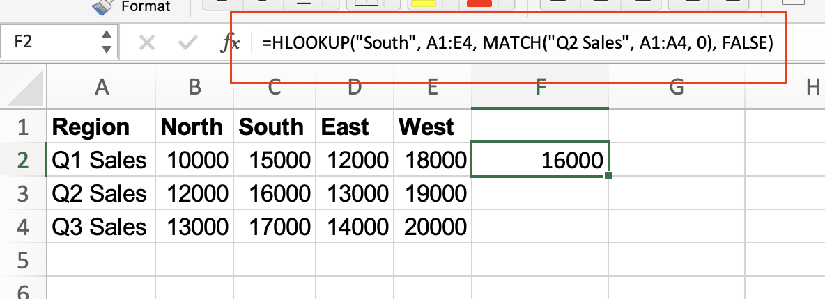
To find Q2 sales for the South region:

=HLOOKUP(“South”, A1:E4, MATCH(“Q2 Sales”, A1:A4, 0), FALSE)

This returns: 16000

Common HLOOKUP Applications

Product Specifications Lookup

Example with computer parts:

Model	i3-9100	i5-9600K	i7-9700K	i9-9900K
Cores	4	6	8	8
Clock	3.6GHz	3.7GHz	3.6GHz	3.6GHz
Cache	6MB	9MB	12MB	16MB

To find the cache size for i7-9700K:

=HLOOKUP(“i7-9700K”, A1:E4, 3, FALSE)

This returns: 12MB

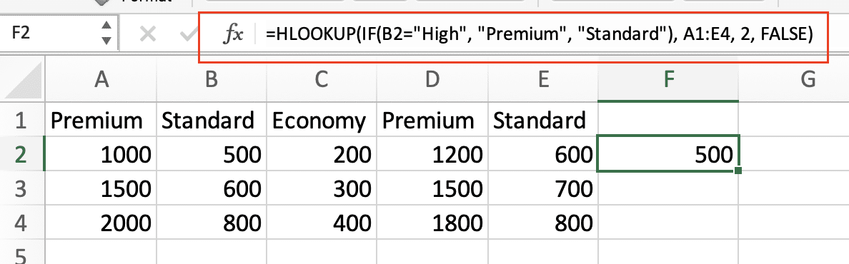
Multiple Criteria Lookups

For complex lookups involving multiple criteria, combine HLOOKUP with IF statements:

=HLOOKUP(IF(B1=”High”, “Premium”, “Standard”), A1:E4, 2, FALSE)

Next Steps

Now that you understand how to use HLOOKUP effectively, you can streamline your data lookup processes and build more efficient spreadsheets. To take your spreadsheet automation to the next level, consider using Coefficient to connect your Excel sheets directly to your data sources, ensuring your lookups always use the most current data.

Ready to automate your spreadsheet data? Get started with Coefficient today →