How to Use GETPIVOTDATA Excel: A Quick Guide

Pivot tables excel at summarizing data, but extracting specific values can be challenging. GETPIVOTDATA addresses this by enabling you to pull exact figures from your pivot tables. This guide will teach you to use GETPIVOTDATA effectively.

We’ll explore its syntax, show real-world applications, and provide troubleshooting tips for common issues. By the end, you’ll be able to swiftly extract precise sales figures, inventory counts, or financial data from your pivot tables for faster reporting.

GETPIVOTDATA 101: The Basics

Let’s break down what GETPIVOTDATA is and why it’s so useful.

The GETPIVOTDATA function retrieves a single, specific value from a Pivot Table based on the criteria you provide.

Here’s the basic syntax:

=GETPIVOTDATA(data_field, pivot_table, [field1, item1, field2, item2], …)

• data_field: The field containing the value you want to retrieve (e.g., “Sales,” “Quantity”).
• pivot_table: A reference to the PivotTable you’re working with.
• [field1, item1, field2, item2], …: Optional arguments specifying the criteria for selecting the data point. You define the field and the corresponding item within that field.

Example:

Let’s say you have a Pivot Table showing sales data by region and product. You want to find the sales figure for “Product A” in the “East” region. The GETPIVOTDATA formula would look something like this:

=GETPIVOTDATA(“Sales”, $A$1:$C$10, “Region”, “East”, “Product”, “Product A”)

This formula tells Excel to look in the PivotTable located in the range $A$1:$C$10, find the “Sales” data field, and return the value where the “Region” is “East” and the “Product” is “Product A.”

Benefits of Using GETPIVOTDATA

The GETPIVOTDATA function offers several key benefits that make it a powerful tool for data analysis in Excel:

1. Flexibility: GETPIVOTDATA allows you to retrieve data from a pivot table based on specific criteria, making it easier to extract the exact information you need for your analysis.
2. Automation: By using dynamic references, GETPIVOTDATA can automatically update as the underlying data or pivot table structure changes, reducing the need for manual updates.
3. Efficiency: GETPIVOTDATA can help you avoid the need to manually navigate through a pivot table or copy and paste data, saving you time and effort.
4. Accuracy: By using GETPIVOTDATA to retrieve data, you can ensure that your analysis is based on the most up-to-date and accurate information from your pivot table.
5. Scalability: GETPIVOTDATA can handle large and complex pivot tables, making it a valuable tool for working with big data sets.

How to Use GETPIVOTDATA in Excel

Using GETPIVOTDATA might seem intimidating at first, but it’s surprisingly straightforward. Let’s walk through a step-by-step example:

1. Create Your PivotTable: Start by creating a PivotTable from your data. This table will be the source for your GETPIVOTDATA function.

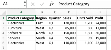
1. Identify Your Target Value: Determine the specific data point you want to extract. What field is it in? What are the corresponding row and column labels?
2. Start Typing Your Formula: In a blank cell, type =GETPIVOTDATA(.

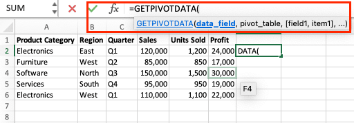
1. Select the Data Field: Select the cell containing the data field you’re interested in (e.g., the cell containing the word “Sales” in your PivotTable).

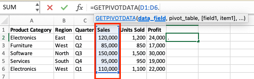
1. Select the PivotTable: Add a comma after the data field and select any cell within your PivotTable.
2. Specify Your Criteria: For each criterion, add a comma after the previous argument and input the following:
   • The field name enclosed in double quotes (e.g., “Region”).
   • A comma.
   • The item name enclosed in double quotes (e.g., “East”).
3. Close the Formula: Close the parentheses and press Enter.

Pro Tip: Excel can often help you build the GETPIVOTDATA formula. As you start typing the formula and select the data field and PivotTable, Excel may suggest arguments based on your PivotTable structure.

Video Tutorial

Advanced GETPIVOTDATA Techniques

Dynamic References with GETPIVOTDATA

One of the most powerful features of the GETPIVOTDATA function is its ability to handle dynamic references. This means that you can use GETPIVOTDATA to retrieve data from a pivot table even as the underlying data changes or the pivot table structure is modified. To leverage dynamic references, you can use cell references or named ranges in your GETPIVOTDATA formula, allowing the function to automatically update as the pivot table is updated.

For example, let’s say you have a pivot table that summarizes sales data by product category and region. You can use a formula like =GETPIVOTDATA(“Sales”, “PivotTable1”, “Product Category”, “Electronics”, “Region”, A2) to retrieve the sales value for the “Electronics” product category and the region specified in cell A2.

As you update the pivot table or change the region in cell A2, the GETPIVOTDATA function will automatically adjust the reference and return the correct value.

Using GETPIVOTDATA with Multiple Criteria

In addition to dynamic references, GETPIVOTDATA also allows you to retrieve data based on multiple criteria. This is particularly useful when you need to analyze data across multiple dimensions, such as product, region, and time period.

To use GETPIVOTDATA with multiple criteria, you can simply add additional arguments to the function, separating each criteria with a comma.

For instance, you could use the formula =GETPIVOTDATA(“Sales”, “PivotTable1”, “Product Category”, “Electronics”, “Region”, “West”, “Quarter”, “Q4”) to retrieve the sales value for the “Electronics” product category, the “West” region, and the “Q4” quarter.

Troubleshooting GETPIVOTDATA Errors

While GETPIVOTDATA is a powerful function, it can sometimes encounter errors or unexpected behavior. Here are some common GETPIVOTDATA errors and how to troubleshoot them:

1. “#REF!” Error: This error typically occurs when the pivot table reference in the GETPIVOTDATA function is no longer valid, often due to changes in the pivot table structure or location. To fix this, ensure that the pivot table name or cell reference is still accurate.
2. “#NAME?” Error: This error can occur when the field names or item names used in the GETPIVOTDATA function are not recognized by the pivot table. Double-check the spelling and capitalization of the field and item names to ensure they match the pivot table exactly.
3. “#VALUE!” Error: This error may appear when the GETPIVOTDATA function is unable to retrieve the requested data, often due to a mismatch between the data types or a lack of data in the specified pivot table location. Verify that the data types and pivot table structure are correct.
4. Incorrect Data Returned: If the GETPIVOTDATA function is returning unexpected or incorrect data, check the following:
   • Ensure that the field and item names in the function are accurate and match the pivot table.
   • Verify that the pivot table filters or slicers are not excluding the data you’re trying to retrieve.
   • Make sure the pivot table is up-to-date and reflects the latest changes in the underlying data.

By understanding these common GETPIVOTDATA errors and following the troubleshooting steps, you can quickly identify and resolve any issues that arise when using this function.

Real-World Applications of GETPIVOTDATA

GETPIVOTDATA is a versatile function that can be applied in a wide range of real-world scenarios. Here are a few examples of how Excel experts and data analysts use GETPIVOTDATA effectively:

Sales Analysis: A sales manager uses GETPIVOTDATA to analyze sales performance by product category, region, and time period. By creating a pivot table and leveraging GETPIVOTDATA, the manager can quickly identify top-selling products, monitor regional trends, and spot any changes in sales patterns over time.

Financial Reporting: An accountant uses GETPIVOTDATA to extract data from a pivot table that summarizes the company’s financial statements, such as income, expenses, and cash flow. This allows the accountant to generate customized reports and perform detailed analyses without having to manually navigate the pivot table.

Marketing Campaign Tracking: A marketing analyst uses GETPIVOTDATA to track the performance of various marketing campaigns, such as email newsletters, social media posts, and paid advertising. By creating a pivot table that consolidates data from multiple sources, the analyst can use GETPIVOTDATA to measure key metrics like click-through rates, conversion rates, and return on investment.

Inventory Management: A supply chain manager uses GETPIVOTDATA to monitor inventory levels and identify trends in product demand. By creating a pivot table that tracks inventory data, the manager can use GETPIVOTDATA to generate reports on stock levels, identify slow-moving items, and optimize inventory replenishment strategies.

Getting More Out of Excel with GETPIVOTDATA and Coefficient

GETPIVOTDATA extracts specific data from pivot tables in Excel. It’s useful but limited to existing spreadsheet data.

Coefficient takes this further by pulling live data from systems like Salesforce or HubSpot straight into Excel. This means your reports always show current sales figures, customer metrics, and marketing data—no manual updates needed.

Ready to expand your Excel toolkit? Get started with Coefficient today for free!