The FV (Future Value) function in Excel helps calculate how much an investment will grow over time. Whether you’re planning retirement savings, analyzing investment returns, or projecting loan payments, mastering this function is essential for financial planning. This guide walks you through every aspect of using the FV function effectively.

How to Calculate Future Value in Excel Using the FV Function

The FV function uses this basic syntax:

=FV(rate, nper, pmt, [pv], [type])

Where:

• rate: Interest rate per period
• nper: Total number of payment periods
• pmt: Regular payment amount
• pv (optional): Present value or starting amount
• type (optional): When payments are due (0 = end of period, 1 = beginning)

Setting Up Your First FV Calculation

Let’s create a basic investment calculation.

Command: Create a new Excel worksheet

1. Open Excel and create a new blank worksheet
2. Label cell A1 as “Investment Calculator”
3. Create the following layout:

Parameter	Value	Description
Interest Rate	5%	Annual interest rate
Years	10	Investment period
Monthly Payment	$100	Regular contribution
Initial Investment	$1,000	Starting amount
Future Value	[Formula]	Calculated result

Command: Enter your first FV formula

1. In the Future Value cell, enter:

=FV(5%/12, 10*12, -100, -1000, 0)

This formula calculates:

• Monthly rate (5%/12)
• Total periods (10 years * 12 months)
• $100 monthly payment
• $1,000 initial investment
• Payments at period end

The result: $17,175.24

Adding Payment Schedules to Your FV Calculations

Let’s explore different payment frequencies.

Command: Create a payment frequency comparison

Create this table:

Payment Frequency	Formula	Result
Monthly	=FV(5%/12, 10*12, -100, -1000, 0)	$17,175.24
Quarterly	=FV(5%/4, 10*4, -300, -1000, 0)	$17,090.49
Annually	=FV(5%, 10, -1200, -1000, 0)	$16,722.37

Creating an Investment Calculator with the FV Function

Let’s build a dynamic calculator.

Command: Set up variable inputs

1. Create input cells:
   • A2: Annual Rate
   • B2: Investment Years
   • C2: Monthly Contribution
   • D2: Initial Amount
2. Create the formula cell with references:

=FV(A2/12, B2*12, -C2, -D2, 0)

Calculating Investment Returns with Multiple Scenarios

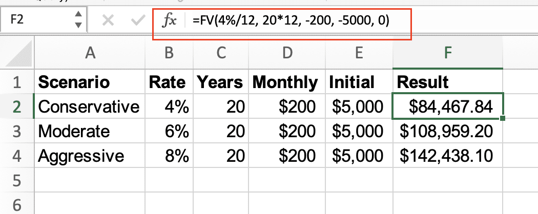
Command: Create a scenario analysis table

Scenario	Rate	Years	Monthly	Initial	Result
Conservative	4%	20	$200	$5000	=FV(4%/12, 20*12, -200, -5000, 0)
Moderate Try the Free Spreadsheet Extension Over 500,000 Pros Are Raving About Stop exporting data manually. Sync data from your business systems into Google Sheets or Excel with Coefficient and set it on a refresh schedule. Get Started	6%	20	$200	$5000	=FV(6%/12, 20*12, -200, -5000, 0)
Aggressive	8%	20	$200	$5000	=FV(8%/12, 20*12, -200, -5000, 0)

Essential FV Function Parameters Explained

Rate Parameter

• Must be consistent with payment period
• For monthly payments: Annual rate/12
• For quarterly payments: Annual rate/4

Example:

=FV(7%/12, 5*12, -100, -1000, 0) // 7% annual rate for monthly calculations

Number of Periods (nper)

• Total payment periods
• Must match rate period frequency
• Years * frequency (12 for monthly, 4 for quarterly)

Payment (pmt)

• Regular payment amount
• Negative for investments (money out)
• Positive for loans (money received)

Optional Parameters and Their Impact

Present Value (pv)

• Initial investment amount
• Negative for investments
• Optional (defaults to 0)

Example with and without PV:

=FV(6%/12, 10*12, -100, 0, 0) // No initial investment

=FV(6%/12, 10*12, -100, -1000, 0) // With $1000 initial investment

Type Parameter

Compare beginning vs end of period payments:

Payment Timing	Formula	Result
End (0)	=FV(6%/12, 10*12, -100, -1000, 0)	$18,207.33
Beginning (1)	=FV(6%/12, 10*12, -100, -1000, 1)	$18,289.27

Real-World Applications of the FV Function

1. Retirement Planning:

=FV(7%/12, 30*12, -500, -10000, 0) // 30-year retirement savings

1. College Fund:

=FV(5%/12, 18*12, -200, -5000, 0) // 18-year education fund

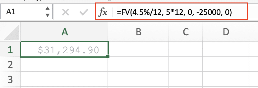
1. Loan Growth:

=FV(4.5%/12, 5*12, 0, -25000, 0) // 5-year loan growth

Ready to enhance your financial modeling capabilities? Coefficient helps you automate these calculations by connecting live data from your financial systems directly to Excel. Start building dynamic financial models with real-time data updates.

Get started with Coefficient today