Understanding The Excel UNIQUE Function

In data analysis, ensuring precision is uppermost, and one significant tool for accomplishing this is the Excel UNIQUE function. The UNIQUE function recovers unique values from a range or array, abolishing any duplicate values. It’s predominant purpose is to provide a clean and brief list of different values, which helps handle the incorporation of your calculations and overall data inspection.

The Excel UNIQUE function retrieves unique values from a range or array, removing any duplicate values.

Its primary purpose is to provide a clean and concise list of distinct values to ensure accuracy during calculations and data analysis.

We’ll dive into how to use it later in the article. But first, let’s examine its syntax.

Syntax Of The Excel UNIQUE Function

The general syntax for the UNIQUE function is: =UNIQUE(array, [by_col], [exactly_once])

Where:

• array is the range of cells that you want to analyze for unique values. It can be a single column, a row, or a more complex array of cells.
• by_col is an optional argument which you can set as TRUE to compare columns against each other and return unique columns. FALSE (or omitted) will compare rows against each other and return unique rows.
• exactly_once is another optional argument which will return distinct rows or columns that occur only once in an array, if defined as TRUE. If defined as FALSE (or omitted), the function returns all distinct rows or columns.

Examples:

Basic Usage:
Extract unique values from a list: =UNIQUE(A1:A10)

Extract Unique Rows:
Extract unique rows from a range of table: =UNIQUE(A1:B10)

Extract Unique Columns:
Extract unique columns from a range of table: =UNIQUE(A1:B10, TRUE)

Return Items Unfolding Exactly Once:
Return items from a list that appears exactly once: =UNIQUE(A1:A10, , TRUE)

Practical Examples:
We have arranged a dataset in cells ‘A1:C5’:

• Extract Unique Rows: =UNIQUE(A1:C5)

Result:

• Extract Unique Columns: =UNIQUE(A1:C5, TRUE)

Result:

• Return values that appear exactly once: =UNIQUE(A1:A10, , TRUE)

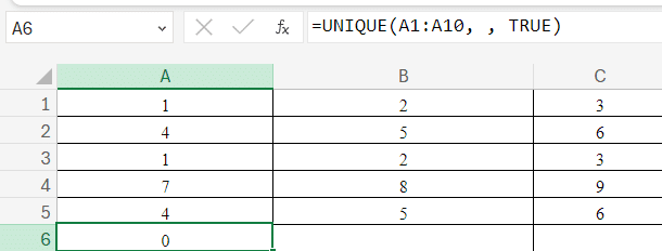
This will be easier to understand with a simple example.

Example Of The Basic Use Of Excel UNIQUE

If you have a list of customer IDs in column B, some of which are repeated, you can use the UNIQUE function to extract a list of unique customer IDs.

The formula for that is: =UNIQUE(B4:B12)

This function returns all unique values in the array B4:B12.

Now, if the customer IDs were in a column, instead of a row, you’d use the formula: =(UNIQUE(B4:J4,TRUE))

This function returns unique customer IDs, but since the array is horizontal, it uses TRUE for the by_col argument.

Instead of viewing unique customer IDs, if you wanted to see a list of customers who have only bought one product (i.e,. only have one entry in the Customer ID column), you’d use the formula: =UNIQUE(B4:B12,FALSE,TRUE)

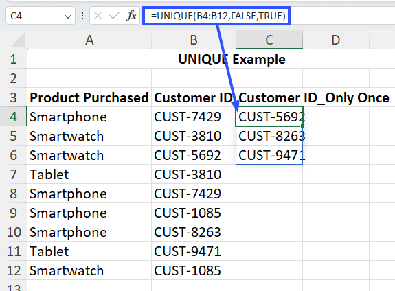
This function returns customer IDs that only occur once in the array B4:B12.

Now that we’ve shown how to use the UNIQUE function in Excel, let’s dive into some tips for optimizing its use.

Tips For Using The Excel UNIQUE Function Effectively

Here’s a set of tips for effectively utilizing the UNIQUE function in Excel:

• Preparation and Planning: Before applying the Excel UNIQUE function, arrange your data so that each type of information (names, dates, etc.) is in a distinct column. This facilitates the effective extraction of unique values.
• Optimize for Large Data Sets: When working with large data sets, keep an eye on performance and optimize your workbook. If necessary, reduce computational demands or split data into smaller segments.
• Data Cleanup: Employ the Excel UNIQUE function as a tool for identifying and eliminating duplicate entries, ensuring the cleanliness and reliability of your data before further analysis.
• Document Your Formulas: When employing the UNIQUE function in complex formulas, document your methods and rationale. Comments within your Excel file can aid you and others in understanding the setup and purpose of your formulas.
• Comprehensive Testing: Ensure that your UNIQUE formula performs as expected across all data scenarios by conducting thorough testing. This will help catch and correct any inconsistencies or errors early on.
• Utilize Dynamic Arrays: If you’re using Excel 365, leverage dynamic arrays to make formulas like UNIQUE more dynamic and flexible. Dynamic arrays auto-expand and adjust as data changes, offering real-time results with minimal manual adjustments.
• Enhance Visibility with Conditional Formatting: Use conditional formatting in conjunction with UNIQUE to highlight unique values in your data set. This makes them easily identifiable and enhances the data’s visual appeal.
• Data Visualization Integration: Use the output from the Excel UNIQUE function as a foundation for charts and graphs to highlight trends and insights that may not be apparent from raw data alone.

With these tips, you can harness the full potential of the UNIQUE function in Excel. So now, let’s look at some advanced use cases for this function.

Advanced Usage Of The Excel UNIQUE Function With Examples

Here are some advanced usage and formula examples of the UNIQUE function in Excel:

Example #1: Extracting Unique Combination Of Values From Multiple Rows (Or Columns)

• If your data is spread across multiple rows (or columns), you can extract the unique combination of all the values spread across them with the UNIQUE function.
• Use the formula: =UNIQUE(A4:B12)
• Where, A4:B12 is the range containing all the values.

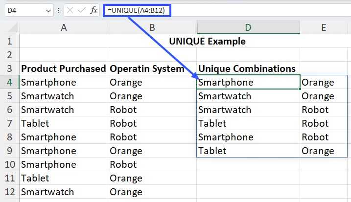
This function has extracted all the unique combinations of Product Purchased and Operating System values.

Example #2: Sorting Unique Values Alphabetically

• If you want to alphabetically sort the unique data you’ve extracted, you can combine the Excel UNIQUE function with SORT.
• The formula would become: =SORT((UNIQUE(A4:B12)))

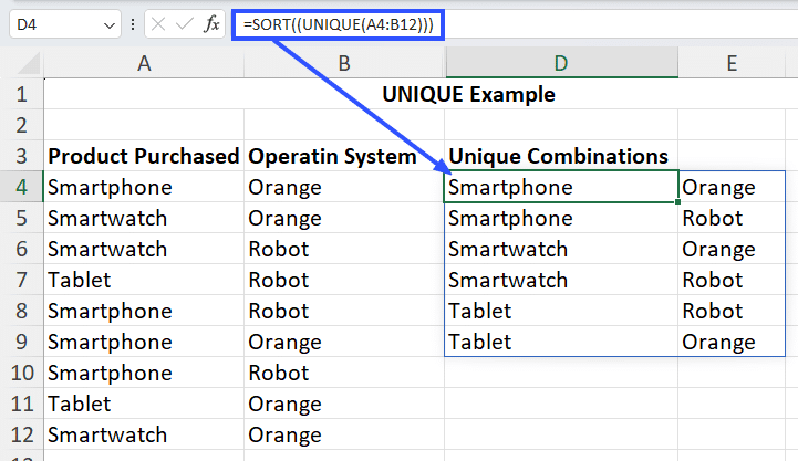
This function results in the unique values in the array A4:B12 sorted alphabetically, based on the values in column A.

Example #3: Concatenating Unique Values From Multiple Columns

• To concatenate unique values from multiple columns, you need to specify each column separately in the array argument, separated by an ampersand (&) symbol.
• The formula looks like this: =UNIQUE(A4:A12&” “&B4:B12)

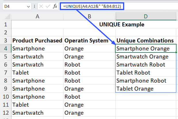
This function concatenates the unique values in the columns A4:A12 and B4:B12, and “ ” adds a space between the two values.

Example #4: Listing Unique Values Based on Specific Criteria

• Let’s say you want to list unique values in an array, but not all of them. To do so, you can use the FILTER function along with the Excel UNIQUE function to specify the criteria.
• The formula to use will be: =UNIQUE((FILTER(A4:C12,D4:D12=H3)))

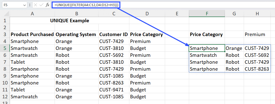
This function extracts all the unique combinations of values in the range A4:C12 which meets the criteria Price Category=Premium.

Try the Free Spreadsheet Extension Over 500,000 Pros Are Raving About

Stop exporting data manually. Sync data from your business systems into Google Sheets or Excel with Coefficient and set it on a refresh schedule.

Get Started

Example #5: Extracting Unique Values Based On Multiple AND/OR Criteria

• You can also use multiple AND or OR criteria to filter the array and extract unique values matching the specified criteria.
• Use the formula: =UNIQUE(FILTER(A4:D12,(D4:D12=H3)+(A4:A12=H4)))

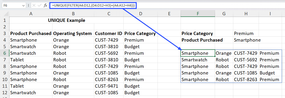
This function extracts all the unique combinations of values in the range A4:D12 which meets the criteria Price Category=Premium OR Product Purchased=Smartphone.

Instead, if you use this formula: =UNIQUE(FILTER(A4:D12,(D4:D12=H3)*(A4:A12=H4)))

Now, the function extracts all the unique combinations of values which meet the criteria Price Category=Premium AND Product Purchased=Smartphone.

Example #6: Ignoring Blank Cells When Finding Unique Values

• If you use the UNIQUE function on an array containing blank cells, the function returns the value 0.

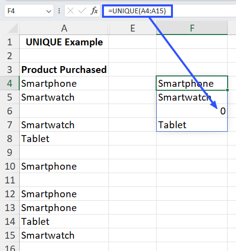
You can exclude blank cells from the array by defining it in the FILTER function with the formula: =UNIQUE(FILTER(A4:A15,A4:A15<>””))

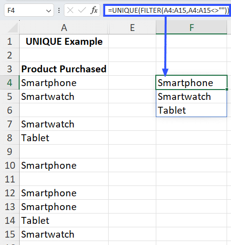
This function uses the condition A4:A15(array)<>(not equal to)“”(blank) to return only the unique values that aren’t blank.

Examples #7: Handling Unique Values In Non-Adjacent Columns

• If you want to extract unique values from columns that are not adjacent, you can combine the Excel UNIQUE function with CHOOSE.
• Here’s the formula to use: =UNIQUE(CHOOSE({1,2},A4:A12,C4:C12))

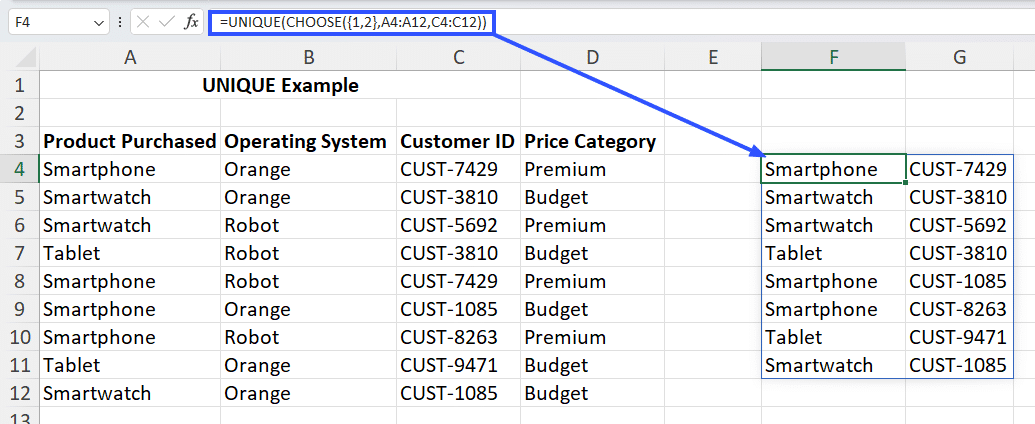
This function uses CHOOSE to define two non-adjacent columns of values and combines it with UNIQUE to return the unique values in the specified columns.

We hope these examples have demonstrated how versatile the Excel UNIQUE function can be, and how it can be combined with other functions to achieve the results you want.

However, you could run into some errors, which you should know how to troubleshoot.

Video Tutorial

Check out the tutorial below for a complete video walkthrough!

How the Excel UNIQUE Function is Useful for Data Analytics Professionals

The Excel UNIQUE Function is a strong tool for data analytics professionals. Here’s why:

Data Refining and Preparation:

• Removing Duplicates: UNIQUE helps in determining and removing duplicate entries from datasets, ensuring that the data is clean and precise.
• Refining Data Sets: It curtails large datasets to their unique components, making it easier to dissect and and demonstrate data.

Data Analysis:

• Determining Unique Values: Helps in rapidly determining unique entries in a column, which is significant for comprehending data distribution and recognizing deviations.

Reporting and Visualization:

• Dynamic Reporting: UNIQUE can be merged with other functions such as SORT and FILTER to create dynamic and communal reports.
• Summary Tables: It assists in creating summary tables that show unique values and their related metrics.

Data Segmentation:

• Market Segmentation: Useful for segmenting the data of customers into different groups based on distinct attributes.
• Product Analysis: Helps in identifying the product lines by recognizing unique product classifications or attributes.

The Excel UNIQUE function is imperative for the data analytics professionals. It improves data refining, streamlines analysis, enhances reporting, enables efficient segmentation, and upgrades performance. By integrating the UNIQUE function into their productivity, data analysts can ensure they operate with clean and effective datasets.

Troubleshooting The UNIQUE Function

Let’s discuss some common errors when using the UNIQUE function in Excel and to fix them:

1. #NAME? error: This error occurs when the function name is misspelled or not recognized by Excel. Fix the spelling to resolve this error.
2. #VALUE! error: This error occurs when the array parameter is not a valid range of cells (e.g., two non-adjacent columns). Define the array parameter with  a valid range of cells to fix this error.
3. #REF! error: You might run into this error when the array argument refers to a range of cells that no longer exist. Redefine array with an updated range of cells to resolve this issue.
4. #SPILL! error: This error occurs when the output array doesn’t fit in the available space. For e.g., when there are non-blank cells in the way of the output array. Clear enough space for the output of the Excel UNIQUE function to fix this error.

Using The Excel UNIQUE Function

The Excel UNIQUE function in Excel is useful for extracting unique values from a range of cells. By manipulating the formula and combining it with other functions, you can extract unique values from multiple rows/columns, concatenate unique values, or extract unique values based on a single/multiple criteria.

When you’re working in a single worksheet, it’s easy to keep track of the behavior and output of the Excel UNIQUE function. But with large data sets across multiple worksheets, all of which are dynamically updated, it can be hard to keep track of.

That’s where Coefficient can make your life easier by connecting all your data sources, automating workflows, and sharing live insights within Excel. Get started with Coefficient today.