Need to quickly pull specific rows or columns from your data? Excel’s TAKE function makes this simple. This guide shows you how to extract exactly the data you need, whether it’s the first few rows of sales figures or the latest customer entries.

How to Extract Data Using the TAKE Function

The TAKE function lets you extract any number of rows or columns from an array. Its simple syntax makes data extraction straightforward:

=TAKE(array, rows, [columns])

Let’s break down each part:

• array: Your source data range
• rows: Number of rows to extract (positive from top, negative from bottom)
• columns: Optional; number of columns to extract

Here’s a basic example:

Name	Sales	Date
John	$1,000	1/1/2025
Sarah	$1,500	1/2/2025
Mike	$2,000	1/3/2025

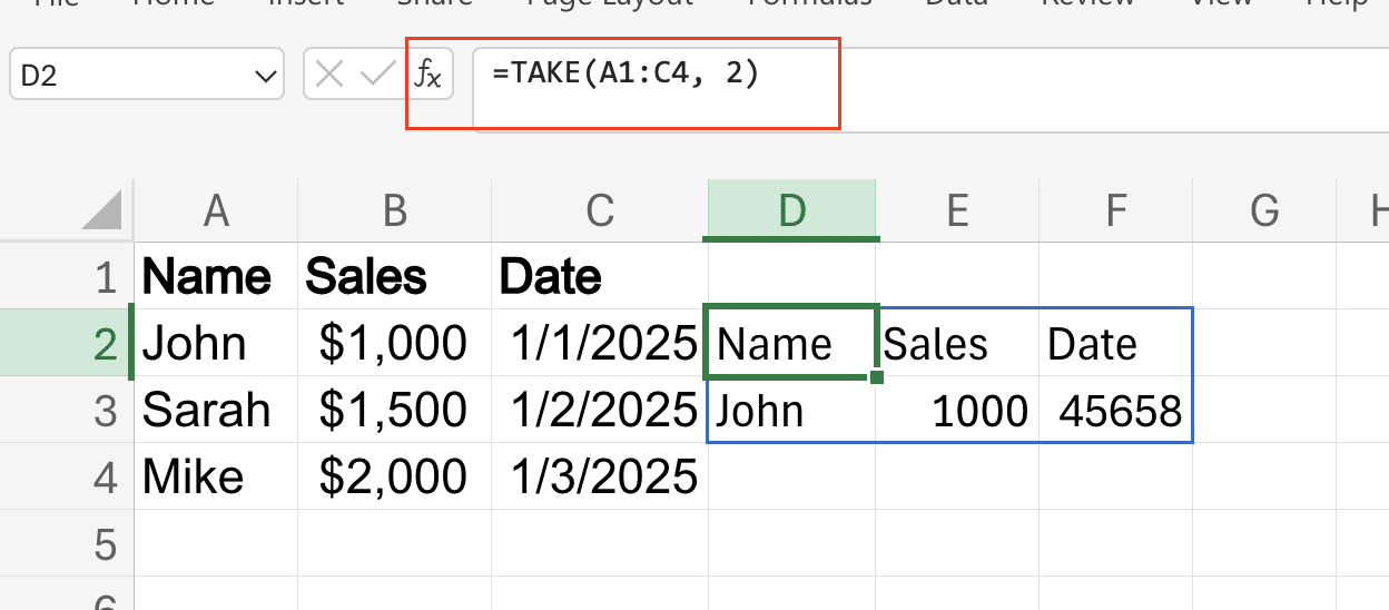
To extract the first two rows:

=TAKE(A1:C4, 2)

Result:

Name	Sales	Date
John	$1,000	1/1/2025
Sarah	$1,500	1/2/2025

Extract the First N Rows from a Dataset

Let’s look at practical examples of extracting rows from the top of your data:

1. Select your data range
2. Type =TAKE(
3. Select your array (e.g., A1:C10)
4. Enter the number of rows you want
5. Close the parenthesis

Pro tip: Use cell references for the row number to make your formula dynamic:

=TAKE(A1:C10, B15)

Pull Data from the Bottom of Your Array

Want the most recent entries? Use negative numbers:

1. Use the same syntax but with a negative row value
2. Example: =TAKE(A1:C10, -3) pulls the last three rows

This works great for:

• Recent transactions
• Latest inventory changes
• Most recent customer interactions

Creating Dynamic Reports with TAKE

Build reports that update automatically:

1. Combine TAKE with TODAY():

=TAKE(SalesData, COUNTIF(DateColumn, TODAY()))

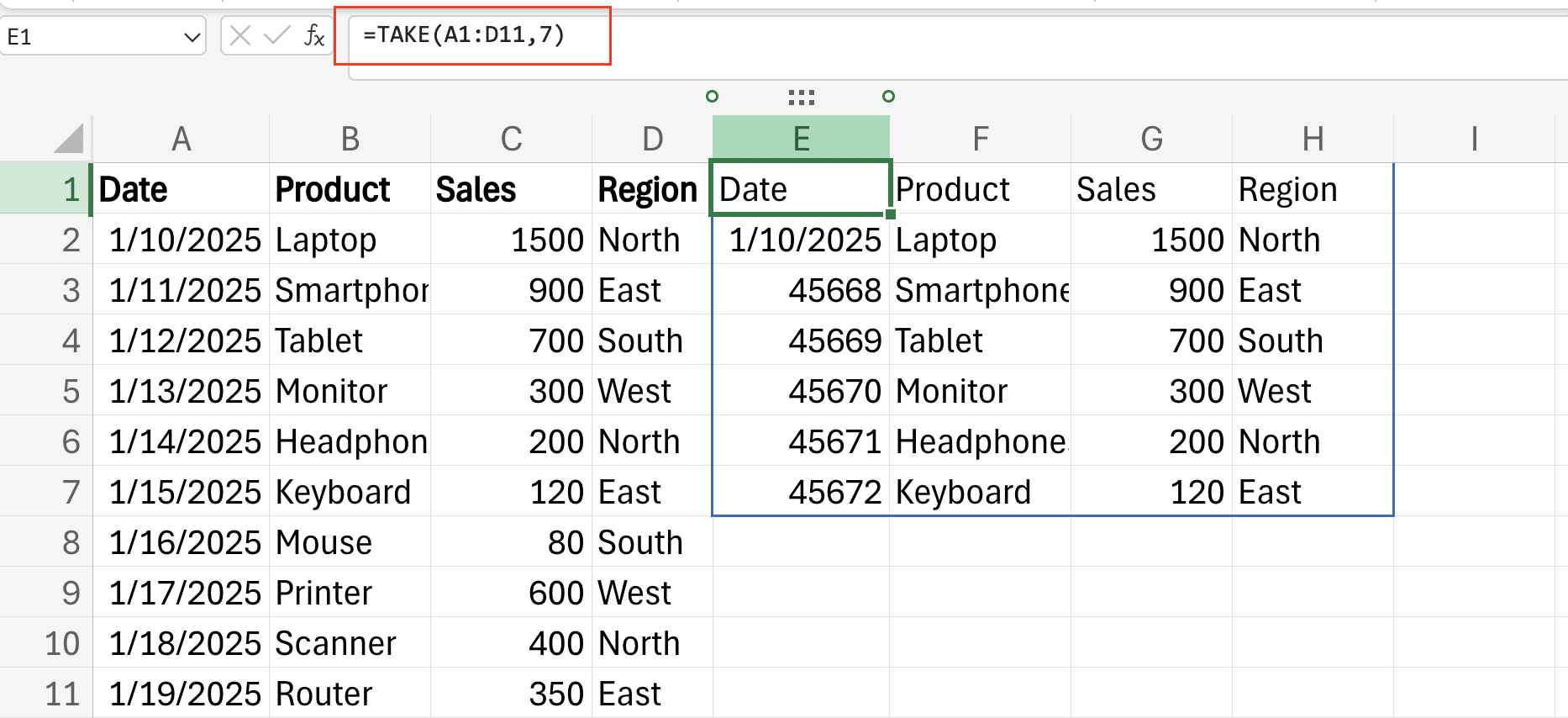
1. Create rolling weekly views:

=TAKE(DataRange, 7)

Column-Based Data Extraction

TAKE handles column selection too:

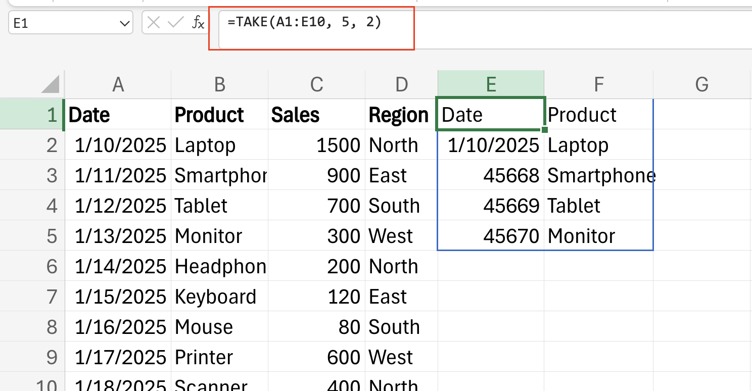
1. Basic column extraction:

=TAKE(A1:E10, 5, 2)

This pulls 5 rows and 2 columns.

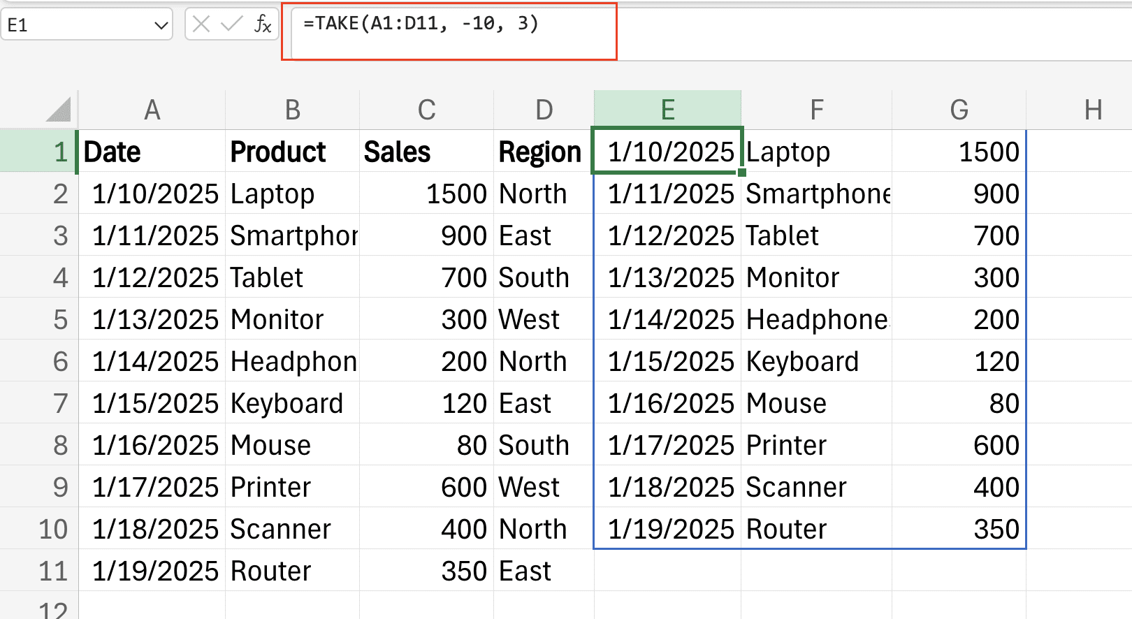
1. Multiple column selection: Use the optional third parameter to specify columns:

=TAKE(FullRange, -10, 3)

TAKE Function in Excel Formulas

Combine TAKE with other functions for powerful results:

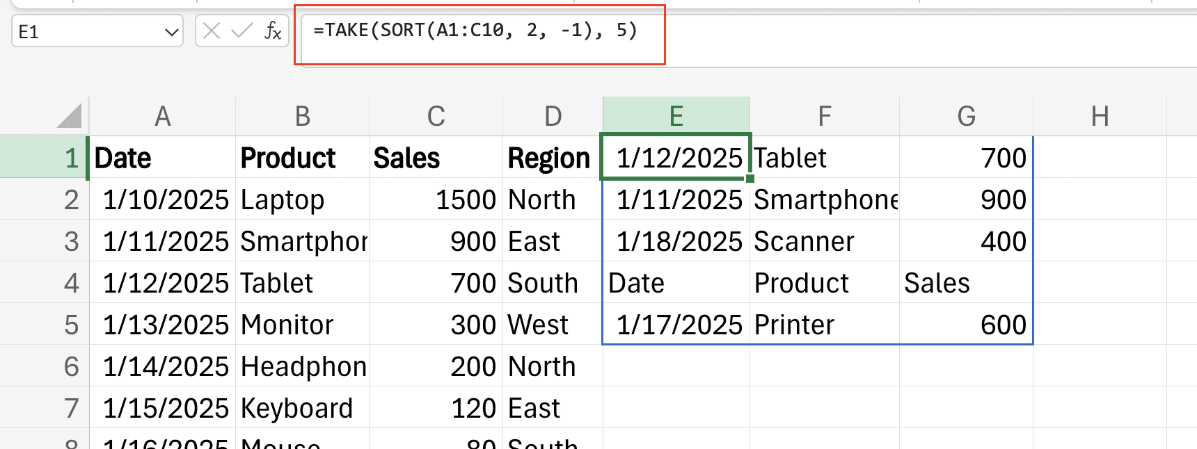
1. With SORT:

=TAKE(SORT(A1:C10, 2, -1), 5)

This sorts by column 2 and takes the top 5 rows.

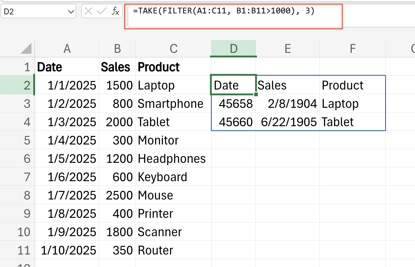
1. With FILTER:

=TAKE(FILTER(A1:C10, B1:B10>1000), 3)

Working with Large Datasets

For big data ranges:

1. Limit your array size
2. Use structured references when possible
3. Consider breaking large ranges into smaller chunks

Alternative Approaches (for Excel 2019 and Earlier)

If you’re using an older Excel version, try these alternatives:

1. OFFSET function:

=OFFSET(A1, 0, 0, 5, 3)

1. INDEX with COUNTA:

=INDEX(A1:C10, ROW(1:5), COLUMN(A:C))

Next Steps

Ready to put the TAKE function to work? Start small with a simple dataset, then build up to more complex extractions.

Want to make your Excel data management even better? Try Coefficient to sync live data directly into your spreadsheets. Get started with Coefficient and transform how you handle data in Excel.

<meta_description> Title: “Excel TAKE Function: Extract Any Data in Seconds (2025 Tutorial)” Description: “Master Excel’s TAKE function with this step-by-step guide. Learn to extract specific rows and columns from arrays with real examples and practical tips.” </meta_description>