
Introduction to the Excel SEARCH and FIND Functions
The Excel SEARCH and FIND functions help you find where certain words or characters are in a text. These functions are useful for pulling specific words from your data or checking if certain words are in your data.
Eager to find out how to use Excel SEARCH function in practice?
Let’s start with the basics.
Understanding the Excel SEARCH Function: Syntax and Differences with FIND
Both these functions are similar, but with slight differences as highlighted below:
| SEARCH | FIND | |
| Syntax | =SEARCH(find_text, within_text, [start_num]) | =FIND(find_text, within_text, [start_num]) |
| Case Sensitivity | Case-Insensitive | Case-Sensitive |
| Wildcards | Supports wildcards (*, ?) | Doesn’t support wildcards |
As you can see from the syntax for both functions, they take identical arguments. These are:
- find_text: The character or substring you want to find/search for.
- within_text: The text string within which you want to find/search for the specific character or substring.
- start_num: An optional argument where you can specify from which position within the within_text string you want to find/search. If omitted from the function, the search starts with the first character of the within_text string.
Let’s dive into some practical examples next to show you how you can use the Excel SEARCH and FIND functions to help with your data sorting and analysis.
Let’s explore some practical examples to get a better understanding of the Excel SEARCH function.
Video Tutorial
Check out the tutorial below for a complete video walkthrough!
Practical Examples Of Using Excel’s SEARCH And FIND Functions
Here are some examples of how to use Excel’s SEARCH and FIND functions:
Example #1: Using Wildcards With The Excel SEARCH Function For Partial Matches.
Utilizing the Excel SEARCH function with wildcards like asterisk (*) and question mark (?) allows for finding partial matches in text strings. But you’ll need to use the SEARCH function as FIND doesn’t support wildcards.
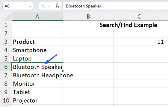
In this example, we’ll use the formula: =SEARCH(“speak*”,A6)
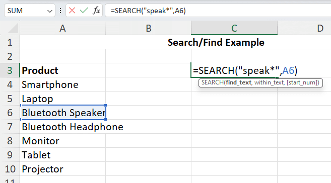
This returns the value 11 as the text string starting with “speak” is located at the 11th position in the search string “Bluetooth Speaker.”
You can use the question mark (?) wildcard in a similar manner.
In our next example, see how the Excel SEARCH function, combined with the FIND and LEFT functions, isolates usernames from email addresses.
Example #2: Extracting A String To The Left Of A Specific Character Using The FIND And LEFT Functions
This example demonstrates using the Excel SEARCH function to define precise extraction points within complex strings
To find text that partly matches, you can use symbols like asterisk (*) and question mark (?) in the SEARCH function.
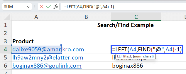
If you have a list of email addresses and you want to get just the usernames: You can accomplish this by using the LEFT function in conjunction with the FIND function.
Use this formula: =LEFT(A4,FIND(“@”,A4)-1)
Let’s break this formula down:
- The LEFT function returns a string from a target string, specified by the number of characters starting from the leftmost character of the target string.
- The LEFT function’s first argument is text, which we’ve defined as A4, where the first email address is located.
- The LEFT function’s second argument is num_chars, which specifies how many characters to extract (starting from the first character).
- To get everything before the ‘@’ symbol, we find where ‘@’ is and subtract 1.. Hence the syntax we use for it is: FIND(“@”,A4)-1.
As you can see, we can just drag the formula down the entire list to retrieve only the username from a list of email addresses.
Example #3: Extracting A String To The Right Of A Specific Character Using The Excel SEARCH And RIGHT Functions
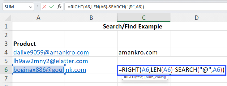
If we take the above example, but want to extract all the domain names from the list of email addresses, we can use the RIGHT function in conjunction with the SEARCH function (could use FIND too).
Since we don’t know how many letters come after the ‘@’, we use the LEN function to count them.
The syntax for this use case is: =RIGHT(A6,LEN(A6)-SEARCH(“@”,A6))
Let’s break this formula down too:
- The RIGHT function returns a string from a target string, specified by the number of characters starting from the rightmost character of the target string.
- The RIGHT function’s first argument is text, which we’ve defined as A6, where the first email address is located.
- The RIGHT function’s second argument is num_chars, which specifies how many characters to extract (starting from the rightmost character).
- But we don’t know the number of characters in the email address, so we use the LEN function to determine it and subtract the number given by the SEARCH function, based on the ‘@’ symbol’s position. So the num_chars argument is defined by LEN(A6)-SEARCH(“@”,A6).
Example #4: Conditional Testing For A Text String Using Excel SEARCH, ISNUMBER, And IF Functions
Conditional testing is another powerful application of the Excel SEARCH function
Let’s say you have a list of email addresses and want to find out which of those are from the domain orange.com.
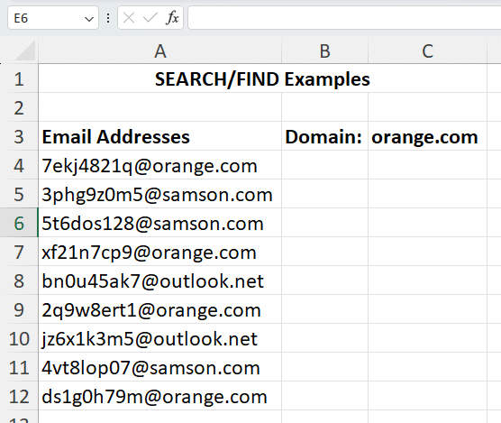
This requires you to check for the presence of the string “orange.com” in each cell in column A.
You can use the ISNUMBER function with the SEARCH function to test if the string “orange.com” is present in the email address in the following way:
- Using the SEARCH function to search for the string “orange.com” within each email address will return a number corresponding to the location of the string within the main text string.
If the string “orange.com” is not present, the SEARCH function will return #VALUE! error. - The ISNUMBER function returns the value TRUE if the cell contains a number. Or else, it returns FALSE.
Hence, you can get the result you want by using the function like this: =ISNUMBER(SEARCH($C$3,A4))
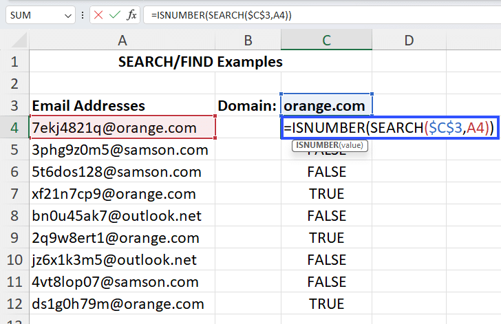
Use the absolute cell reference for cell C3, then drag this formula down the whole column. This will result in TRUE against all email addresses that contain the string “orange.com.”
You can also use the IF function with ISNUMBER and SEARCH to output a more customized value, like so: =IF(ISNUMBER(SEARCH($C$3,A4)),”Orange Customer”,”Other Customer”)
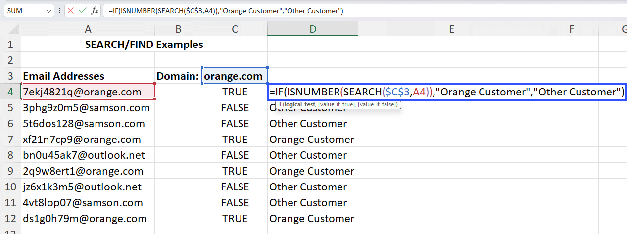
With this function, you’ll get the output “Orang Customer” when the ISNUMBER function returns TRUE. If the ISNUMBER function returns FALSE, the output will be “Other Customer.”
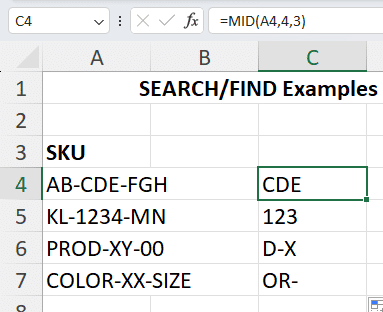
Example #5: Extracting A String Between Two Characters Using Excel SEARCH/FIND And MID Functions
Let’s say you have a list of SKUs for various products and the characters between the two hyphens (-) denote the product specification, which you want to know. You can use the MID function to extract that specific string.
The syntax for it is : =MID(A4,4,3)
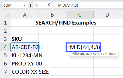
The start_num argument is 4, which is the location of the first hyphen+1; the num_chars argument is 3, which is the number of characters you want to extract from the first SKU.
But this will only work for the first SKU, since the location of the first hyphen is different for each SKU. The number of characters between the two hyphens is also different for each SKU. So using the same formula will not give the results you want.
Therefore, you need to use the SEARCH/FIND function to define the start_num and num_chars arguments for the MID function. Let’s do it step by step:

Stop exporting data manually. Sync data from your business systems into Google Sheets or Excel with Coefficient and set it on a refresh schedule.
Get Started
Step 1: To define the start_num argument, you need to find the position of the first hyphen (-) and add 1 to it. So the start_num argument becomes: FIND(“-“,A4)+1 (where A4 refers to the cell which contains the string within which you want to find the hyphen).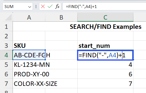
This function returns the value 4, which is the position of the character immediately after the first instance of the hyphen (-) character in cell A4.
Step 2: To define the num_chars argument, you need to find the position of the second hyphen and count the number of characters between the two hyphens
First, you need to find the second instance of the hyphen. But the FIND (and SEARCH) functions only find the first instance of the character. So we need to define the FIND function such that it starts searching the within_text string after the first hyphen.
To do so, we’ll define the start_num argument for the FIND function ;to start the search after the first instance of hyphen. This means finding the position of the first hyphen and adding 1 to it.
So the formula to find the second hyphen’s position is: =FIND(“-“,A4,FIND(“-“,A4)+1)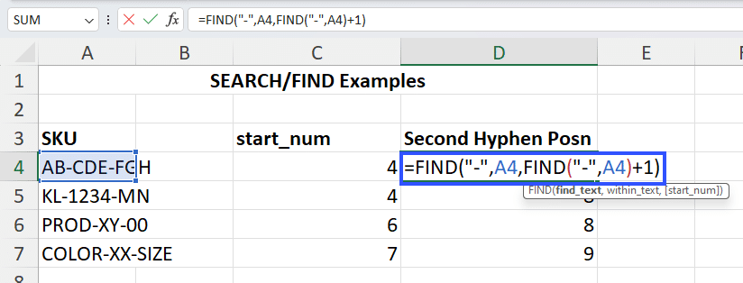
This formula returns the value 7, which is the position of the second hyphen in cell A4.
Step 3: Next, you need to find the number of characters between the two hyphens, so you can define the num_chars argument for the MID function. To do so, you just need to subtract the start_num value from the second hyphen position value.
The formula will then become: =(FIND(“-“,A4,FIND(“-“,A4)+1))-(FIND(“-“,A4)+1)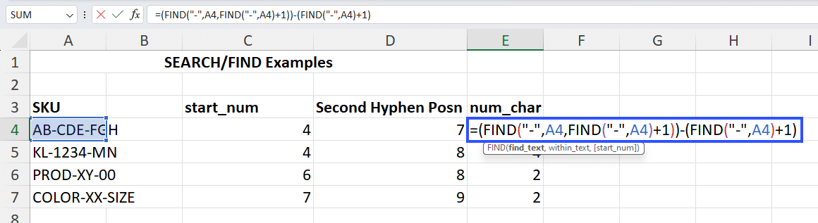
This formula returns the value 3, which is the number of characters between the two hyphens in cell A4.
Step 4: Now that you’ve determined all the arguments for the MID function, it’s time define the function as: =MID(A4,C4,E4)
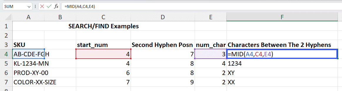
This formula returns the string “CDE.”
This function takes advantage of the values you calculated earlier and uses the cell references in the arguments for the MID function. However, you can also calculate each argument for the MID function within the function itself.
So the formula will become: =MID(A4,FIND(“-“,A4)+1,(FIND(“-“,A4,(FIND(“-“,A4)+1))-(FIND(“-“,A4)+1)))
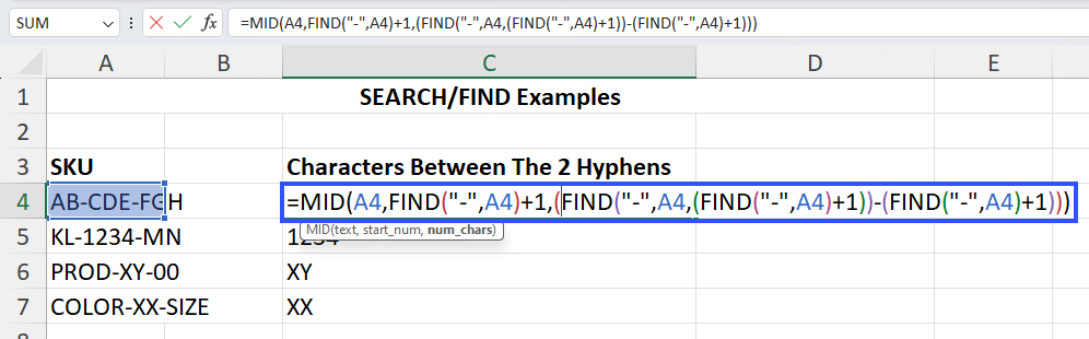
This formula returns the string “CDE.”
You can just drag this formula down the entire column to extract the string between the 2 hyphens in the SKU column.
Example #6: Using the SEARCH Function in the Formula
If you want to locate the rows where the department is “IT” using a formula, you can use the ‘SEARCH’ function in amalgamation with other functions such as ‘IF’.
First, add a new column for the search results: Let’s use the E Column for this intention. In E2 Cell, enter this formula:
=IF(ISNUMBER(SEARCH(“IT”, C2)), “Found”, “Not Found”)
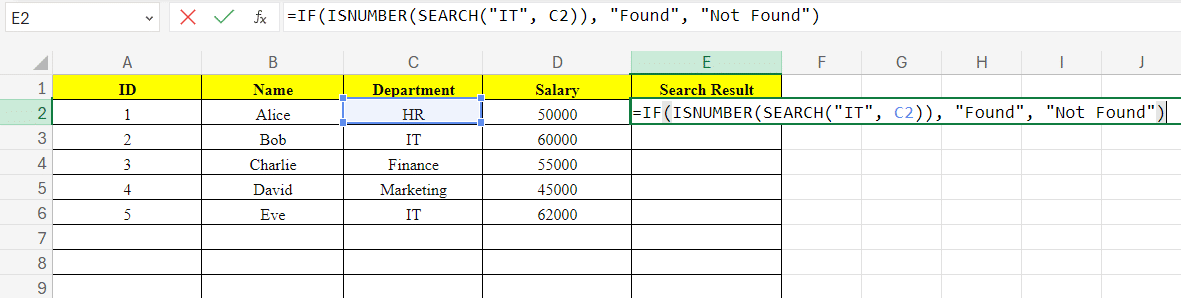
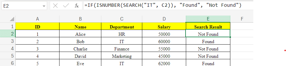
Then, copy the Formula Down: Haul the fill handle from E2 to E6 to imply the formula to all the rows.
The outcome will look like this:
Using The Excel SEARCH And FIND Functions
This comprehensive guide illustrates various ways to leverage the Excel SEARCH function to simplify data manipulation tasks.
If you’ve ever found yourself sifting through endless rows of data, attempting to pinpoint specific information with the Excel SEARCH and FIND functions, you know how time-consuming and error-prone manual data extraction can be. Imagine replacing hours of frustration with a few clicks and letting an advanced tool handle the heavy lifting. That’s where Coefficient comes in.
Don’t let repetitive tasks drain your productivity. Embrace the power of automation with Coefficient, the ultimate sidebar app for Excel, and transform how you work. Ready to make the switch? Start your journey towards efficiency today!


