The LARGE function in Excel helps you find specific ranked values within your dataset. Whether you need the highest, second-highest, or nth highest value, this function provides a straightforward way to analyze your data. Let’s explore how to use LARGE effectively through practical examples and real-world applications.

Finding Specific Ranked Values with LARGE Function

The LARGE function uses two simple parameters: array and k. Here’s the basic syntax:

=LARGE(array, k)

Where:

• array: The range of numbers to evaluate
• k: The position from largest (1 for largest, 2 for second-largest, etc.)

Let’s work through a practical example:

1. Create a sample dataset:

A1: Sales Data

A2: 1500

A3: 2300

A4: 1800

A5: 3200

A6: 2700

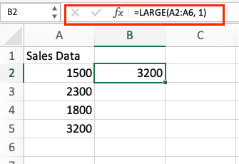
1. Find the largest value:

=LARGE(A2:A6, 1)

Result: 3200

Getting the Highest Value in a Dataset

To find the highest value:

1. Select the cell where you want the result
2. Type =LARGE(
3. Select your data range
4. Type ,1)
5. Press Enter

Example with cell references:

=LARGE(B2:B10, 1)

Pro tip: Always use absolute references ($B$2:$B$10) when ing formulas across multiple cells.

Finding Second and Third Largest Values

To find multiple ranked values:

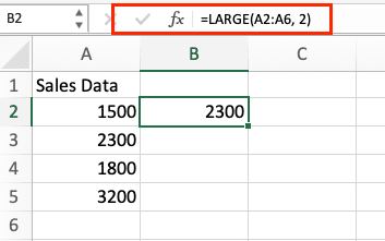
1. For second largest:

=LARGE(A2:A6, 2)

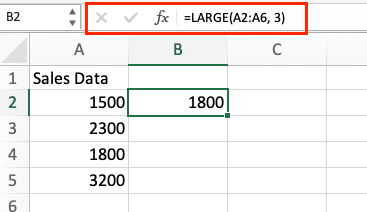
1. For third largest:

=LARGE(A2:A6, 3)

Business example using sales data:

Month	Sales	Rank	Formula
Jan	50000	1	=LARGE($B$2:$B$13, 1)
Feb	45000	2	=LARGE($B$2:$B$13, 2)
Mar	42000	3	=LARGE($B$2:$B$13, 3)

Combining LARGE with Other Excel Functions

LARGE becomes more powerful when combined with other functions:

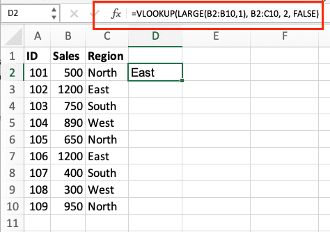
1. With VLOOKUP:

=VLOOKUP(LARGE(B2:B10,1), B2:C10, 2, FALSE)

This formula finds the highest value and returns corresponding data from another column.

1. With INDEX/MATCH:

=INDEX(A2:A10, MATCH(LARGE(B2:B10,1), B2:B10, 0))

This returns the name/label associated with the largest value.

Working with Multiple Data Ranges

To compare across different ranges:

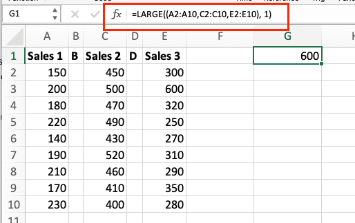
1. Consolidate ranges:

=LARGE((A2:A10,C2:C10,E2:E10), 1)

1. Use array formulas:

=LARGE(IF(A2:A10>=0,A2:A10,””), 1)

Creating Dynamic Top-N Reports

Build flexible ranking systems:

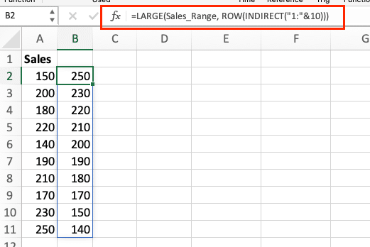
1. Create a parameter cell for N
2. Use dynamic ranges:

=LARGE(Sales_Range, ROW(INDIRECT(“1:”&N)))

Real-world application:

• Monthly top performers
• Highest revenue products
• Best-selling items

Handling Non-Numeric Data

To manage data quality:

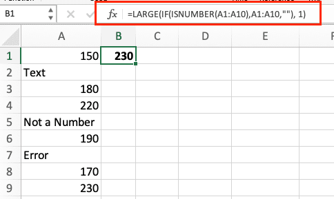
1. Remove errors:

=LARGE(IF(ISNUMBER(A2:A10),A2:A10,””), 1)

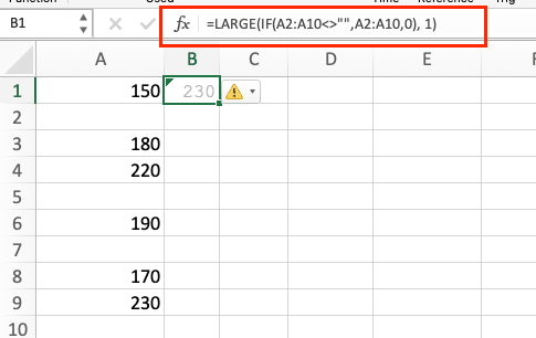
1. Handle blank cells:

=LARGE(IF(A2:A10<>””,A2:A10,0), 1)

Understanding LARGE Function Mechanics

Key capabilities:

• Processes up to 255 items
• Ignores text and logical values
• Treats FALSE as 0 and TRUE as 1

Limitations:

• Can’t handle array results directly
• Requires numeric values
• Performance impacts with large datasets

LARGE vs SMALL Function Comparison

Feature	LARGE	SMALL
Purpose	Finds nth largest	Finds nth smallest
Syntax	=LARGE(array,k)	=SMALL(array,k)
K value	1 = largest	1 = smallest

Next Steps

The LARGE function excels in creating ranked lists, identifying top performers, and analyzing trends in your data. Master these techniques to build more sophisticated Excel solutions for your business needs.

Ready to take your Excel data analysis to the next level? Try Coefficient to automate your reporting and create dynamic dashboards with real-time data integration.