The AND function in Excel serves as a fundamental tool for testing multiple conditions simultaneously. Whether you need to validate data entry, filter complex datasets, or create dynamic reports, mastering the AND function will help you build more sophisticated spreadsheet solutions.
In this comprehensive guide, you’ll learn how to implement AND functions effectively, from basic syntax to advanced applications.
Create Your First AND Function in Excel
The AND function returns TRUE when all specified conditions are met and FALSE when any condition fails. Let’s start with the basics.
Basic Syntax:
=AND(logical1, [logical2],…)
Step-by-Step: Create a Simple AND Function
- Open a new Excel worksheet
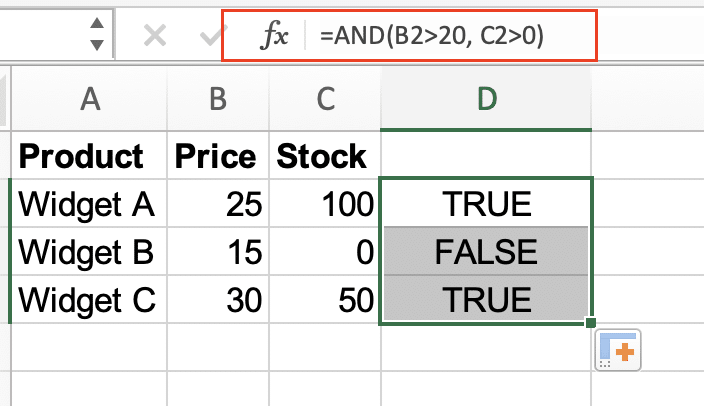
- Enter the following sample data in cells A2:B4:
|
Product |
Price |
Stock |
|---|---|---|
|
Widget A |
25 |
100 |
|
Widget B |
15 |
0 |
|
Widget C |
30 |
50 |
- In cell D2, enter this formula:
=AND(B2>20, C2>0)
This checks if the price is over 20 AND stock is available.
Common Pitfalls to Avoid:
- Don’t forget commas between conditions
- Ensure all referenced cells contain valid data
- Test edge cases with extreme values
How to Combine IF and AND Functions
Combining IF and AND creates powerful conditional logic for decision-making in your spreadsheets.
Creating an IF AND Formula
- Basic syntax structure:
=IF(AND(condition1,condition2),value_if_true,value_if_false)
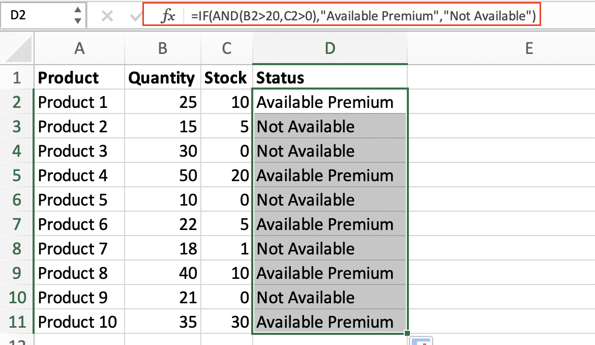
- Practical example using our previous dataset:
=IF(AND(B2>20,C2>0),”Available Premium”,”Not Available”)
Pro Tips:
- Keep conditions simple and readable
- Test each condition separately first
- Use cell references instead of hard-coded values
Testing Multiple Conditions with AND
The AND function can evaluate up to 255 conditions. Here’s how to work with multiple criteria effectively.
Multi-Condition Example:
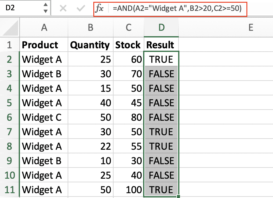
- Create a formula testing three conditions:
=AND(A2=”Widget A”,B2>20,C2>=50)
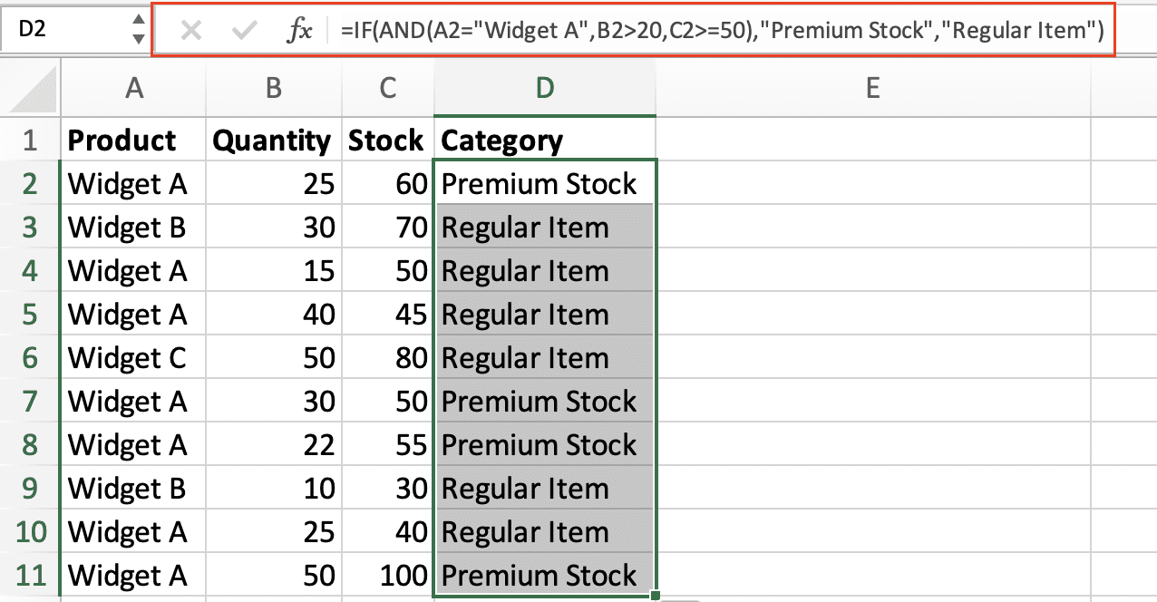
- Combine with IF for meaningful output:
=IF(AND(A2=”Widget A”,B2>20,C2>=50),”Premium Stock”,”Regular Item”)

Stop exporting data manually. Sync data from your business systems into Google Sheets or Excel with Coefficient and set it on a refresh schedule.
Get Started
How to Use AND in Conditional Formatting
Create dynamic visual cues based on multiple conditions.
- Select your data range
- Navigate to Home > Conditional Formatting > New Rule

- Choose “Use a formula“
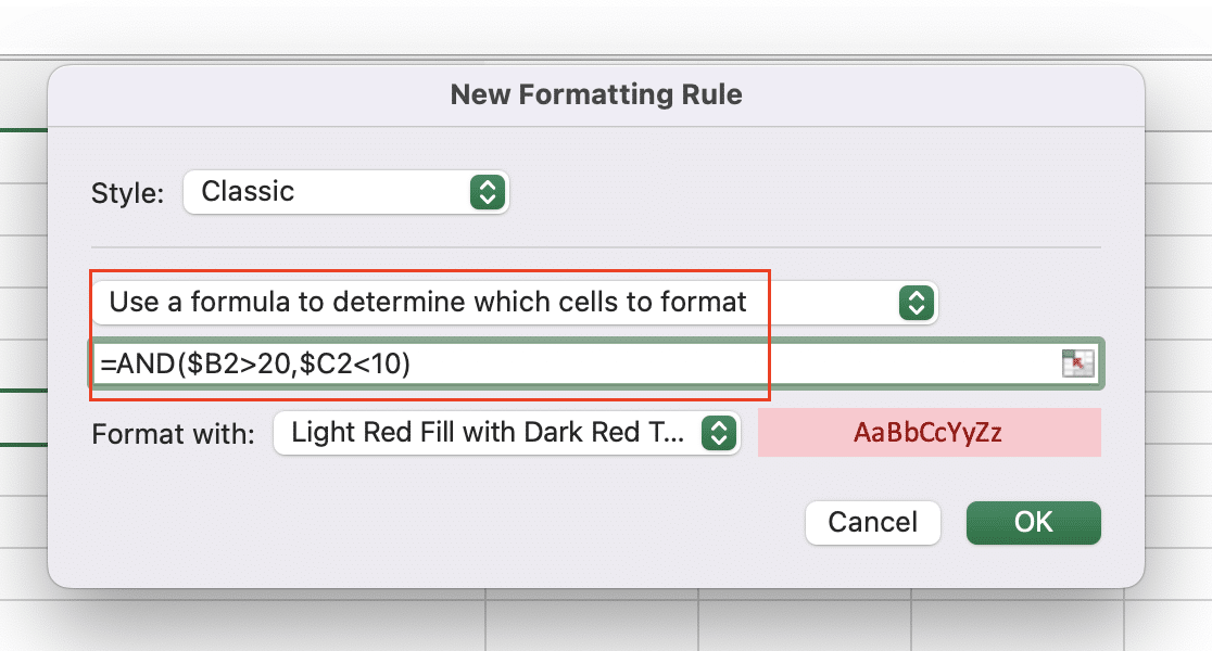
- Enter your AND formula:
=AND($B2>20,$C2<10)
Working with Text Conditions in AND Functions
Text comparisons require careful attention to case sensitivity and exact matches.
Best Practices:
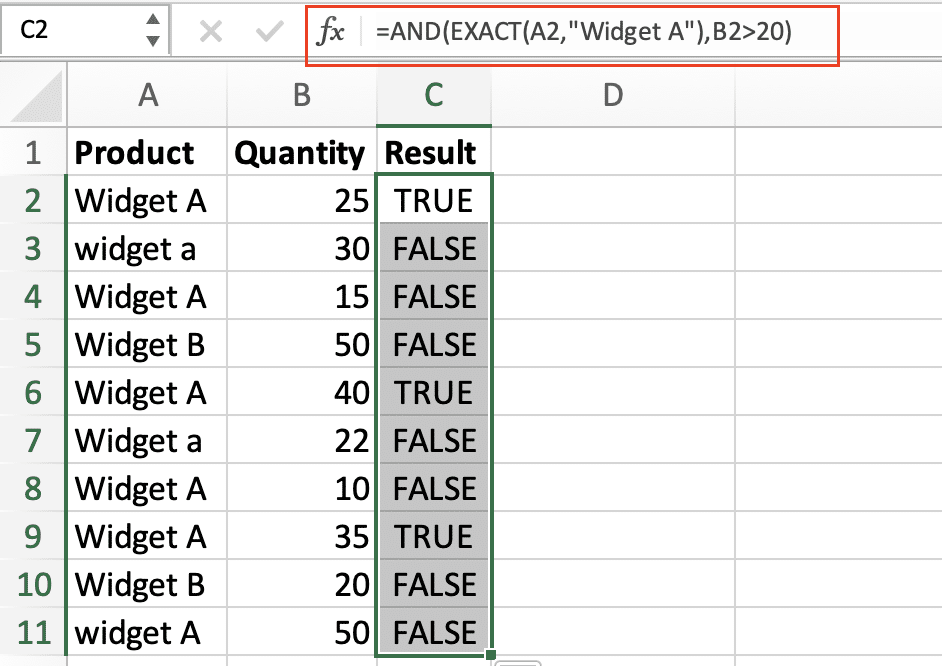
- Use EXACT() for case-sensitive comparisons
- Trim spaces with TRIM()
- Convert case with UPPER() or LOWER()
Example:
=AND(EXACT(A2,”Widget A”),B2>20)
Practical AND Function Examples
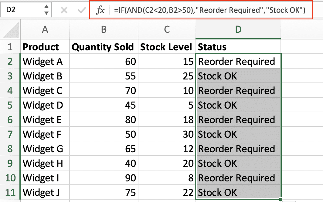
Inventory Management
=IF(AND(C2<20,B2>50),”Reorder Required”,”Stock OK”)
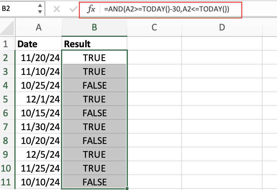
Date-Based Filtering
=AND(A2>=TODAY()-30,A2<=TODAY())
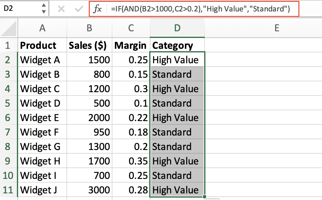
Financial Calculations
=IF(AND(B2>1000,C2>0.2),”High Value”,”Standard”)
Next Steps
Now that you understand how to implement AND functions effectively, experiment with different combinations in your own spreadsheets. Start with simple conditions and gradually build more complex formulas as you become comfortable with the syntax and logic.
For more advanced data management solutions, consider automating your spreadsheet workflows with Coefficient. Get started with Coefficient to seamlessly sync your business data and create real-time reports that update automatically.

