Excel users often struggle with complex data lookups, especially when dealing with large datasets or multiple search criteria. While VLOOKUP is popular, combining INDEX and MATCH functions offers greater flexibility and reliability for data analysis. This tutorial will show you how to master INDEX-MATCH combinations for powerful, dynamic lookups in Excel.

Understanding INDEX and MATCH Functions for Data Lookup

Before combining these functions, let’s understand each component:

The INDEX Function

The INDEX function returns a value from a range based on row and column positions.

Syntax:

=INDEX(array, row_num, [column_num])

Example:

To get the price of Orange:

=INDEX(B2:B4, 2)

Result: 2.49

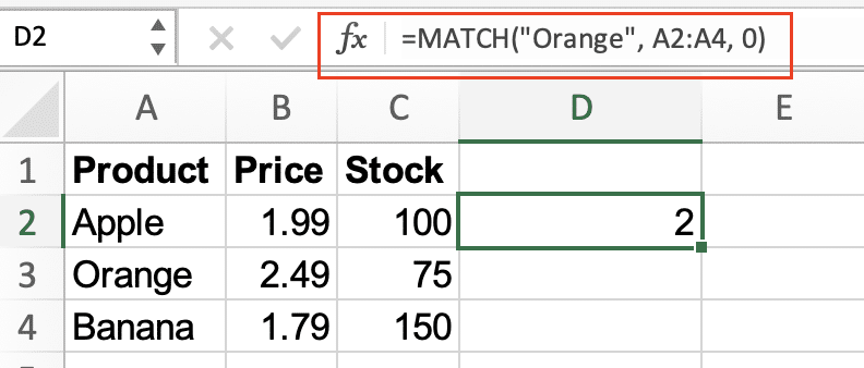
The MATCH Function

MATCH returns the position of a value within a range.

Syntax:

=MATCH(lookup_value, lookup_array, [match_type])

Example using the same table:

=MATCH(“Orange”, A2:A4, 0)

Result: 2 (second position in the range)

Create Your First INDEX-MATCH Formula

Let’s build a basic INDEX-MATCH combination step by step.

1. Set up your data Create a table with sample data:

1. Build the formula To find Mary’s salary:

=INDEX(C2:C4, MATCH(“Mary”, A2:A4, 0))

The formula breaks down as:

• MATCH finds Mary’s position (2)
• INDEX returns the value from the salary column at position 2

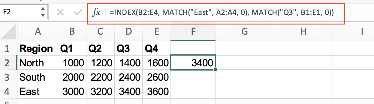
Adding Column References for Two-Way Lookups

For more complex scenarios, you can use two MATCH functions within INDEX.

Example table:

Region	Q1	Q2	Q3	Q4
North	1000 Try the Free Spreadsheet Extension Over 500,000 Pros Are Raving About Stop exporting data manually. Sync data from your business systems into Google Sheets or Excel with Coefficient and set it on a refresh schedule. Get Started	1200	1400	1600
South	2000	2200	2400	2600
East	3000	3200	3400	3600

To find East’s Q3 sales:

=INDEX(B2:E4, MATCH(“East”, A2:A4, 0), MATCH(“Q3”, B1:E1, 0))

Working with Large Datasets

When handling extensive data, consider these optimization techniques:

1. Name Your Ranges Instead of using cell references:

=INDEX(SalesData, MATCH(EmployeeName, EmployeeList, 0))

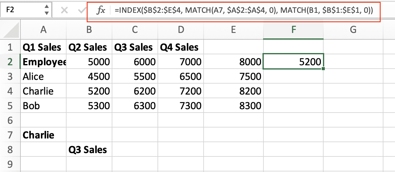
1. Use Absolute References

=INDEX($B$2:$E$4, MATCH(A7, $A$2:$A$4, 0), MATCH(B1, $B$1:$E$1, 0))

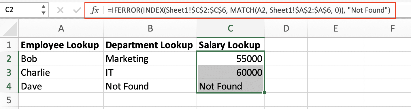
1. Error Handling Add IFERROR to manage missing data:

=IFERROR(INDEX(DataRange, MATCH(Lookup_Value, Lookup_Range, 0)), “Not Found”)

Real-World Applications

Sales Data Analysis

=INDEX(Sales_Data, MATCH(Rep_Name, Sales_Reps, 0), MATCH(Month, Months_List, 0))

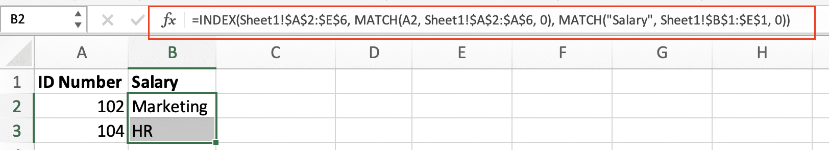
Employee Database

=INDEX(Employee_Data, MATCH(ID_Number, ID_List, 0), MATCH(“Salary”, Field_Names, 0))

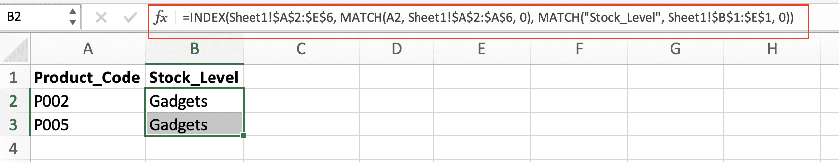
Inventory Management

=INDEX(Inventory, MATCH(Product_Code, Product_List, 0), MATCH(“Stock_Level”, Column_Headers, 0))

Making Your Formulas More Reliable

1. Use Data Validation

• Create dropdown lists for lookup values
• Prevent manual entry errors
• Ensure consistent data format

1. Implement Error Checking

=IF(COUNTIF(Lookup_Range, Lookup_Value)>0,

INDEX(Data_Range, MATCH(Lookup_Value, Lookup_Range, 0)),

“Value not found”)

1. Regular Formula Auditing

• Use Excel’s Formula Auditing tools
• Check for broken references
• Verify range names

Next Steps

Now that you understand how to combine INDEX and MATCH functions effectively, start implementing these techniques in your own spreadsheets. Remember to start with simple lookups before advancing to more complex combinations.

Need to streamline your data management even further? Try Coefficient to automatically sync your business data directly into Excel and create real-time dashboards without complex formulas. Get started with Coefficient today and transform how you work with data in spreadsheets.