
Open your Excel spreadsheet containing duplicate data and ensure it’s organized in a tabular format with clear column headers
Select the cell where you want the combined data to appear (this will be the top-left corner of your consolidated data range)
Click on the “Data” tab in the Excel ribbon, look for the “Data Tools” group and click on the “Consolidate” button
Click “OK” to combine duplicates and sum their values – Excel will create a new consolidated table with unique entries and summed values for duplicates
Combining duplicates in Excel streamlines data management and improves spreadsheet organization. Learn six powerful techniques to merge duplicate entries effectively.
How to Combine Duplicates in Excel Using the Consolidate Function
The Consolidate function in Excel offers a straightforward way to combine duplicates and sum their values. Here’s how to use it:
Step 1: Open your Excel spreadsheet containing duplicate data.
- Launch Excel and open the workbook with the data you want to consolidate.
- Ensure your data is organized in a tabular format with clear column headers.
Step 2: Select the cell where you want the combined data to appear.
- Choose an empty cell in your worksheet where the consolidated data will be placed.
- This cell will be the top-left corner of your consolidated data range.
Step 3: Access the Consolidate feature.
- Click on the “Data” tab in the Excel ribbon.

- Look for the “Data Tools” group and click on the “Consolidate” button.

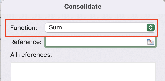
Step 4: Choose the function for combining duplicates.
- In the Consolidate dialog box, click the “Function” drop-down list.
- Select “Sum” from the available options to add up values from duplicate entries.
Step 5: Select the range of cells containing your data.
- Click the collapse dialog button next to the “Reference” field.
- Highlight the range of cells that includes your data, including headers.
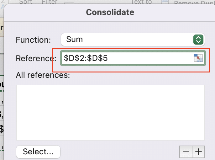
- Click the expand dialog button to return to the Consolidate dialog box.
Step 6: Set up labels and click OK.
- Check the boxes for “Top row” and “Left column” if your data has labels.
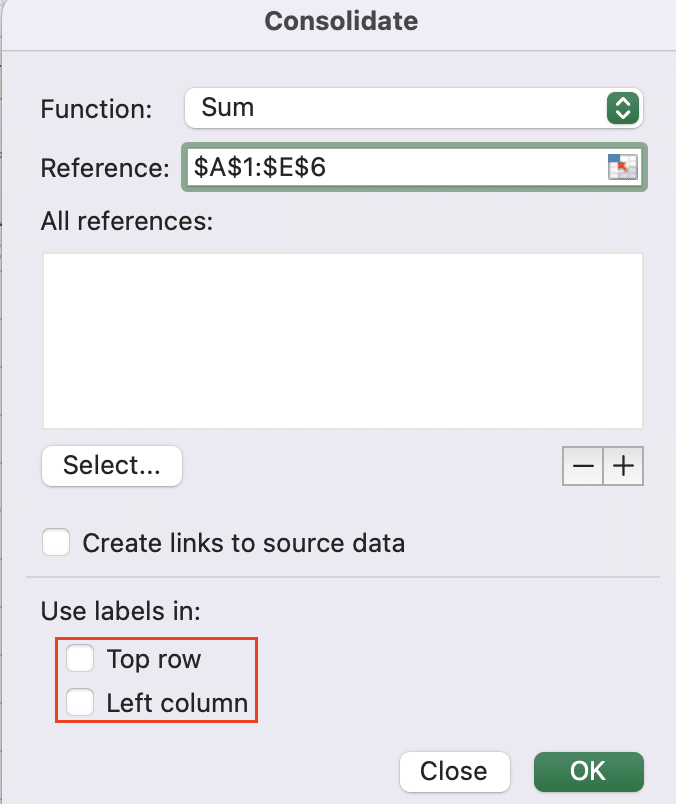
- Click “OK” to combine duplicates and sum their values.
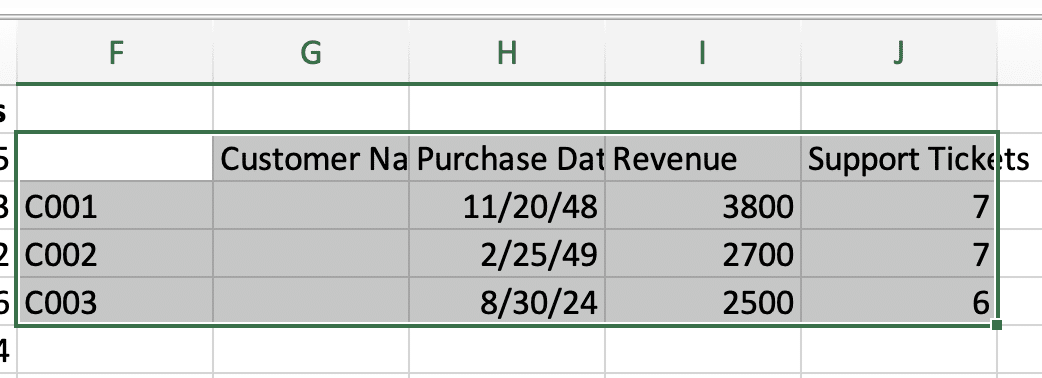
After completing these steps, Excel will create a new consolidated table with unique entries and summed values for duplicates.
Merging Duplicate Rows with Unique Identifiers
When dealing with duplicate rows that have unique identifiers, you can use a combination of Excel functions to merge them effectively:
Step 1: Identify the column containing unique identifiers.
- Locate the column in your dataset that contains unique values for each entry (e.g., Customer ID).
- This column will be the basis for identifying and merging duplicates.
Step 2: Use the Remove Duplicates feature.
- Select your entire data range.
- Go to the “Data” tab and click “Remove Duplicates” in the “Data Tools” group.

- Choose only the column with unique identifiers and click “OK.“
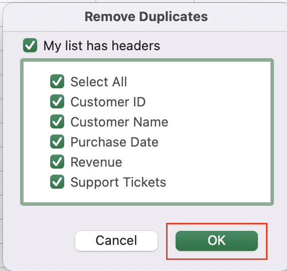
- This action keeps one instance of each unique entry.
Step 3: Employ the VLOOKUP function to retrieve data.
- In a new column, use VLOOKUP to fetch data from the original dataset.
- The formula will look like this: =VLOOKUP(A2,OriginalData!$A$2:$Z$1000,2,FALSE)

- Replace “A2” with your unique identifier cell, “OriginalData” with your sheet name, and adjust the range and column index as needed.
Step 4: Utilize the TEXTJOIN function for text data.
- For text fields that you want to combine, use TEXTJOIN: =TEXTJOIN(“, “, TRUE, FILTER(OriginalData!B$2:B$1000, OriginalData!A$2:A$1000=A2))

- This formula combines all text entries for each unique identifier, separated by commas.
Step 5: Apply the SUM function for numerical values.
- For numerical data, use SUM with FILTER: =SUM(FILTER(OriginalData!C$2:C$1000, OriginalData!A$2:A$1000=A2))

- This calculates the total of all numerical values associated with each unique identifier.
By following these steps, you’ll create a new dataset with merged duplicate rows, maintaining unique identifiers and combining or summing associated data as needed.
Combining Duplicates Using Power Query
Power Query is a powerful tool in Excel for data transformation, including combining duplicates. Here’s how to use it:
Step 1: Open Power Query Editor.
- Click on the “Data” tab in the Excel ribbon.

- Select “From Table/Range” in the “Get & Transform Data” group.
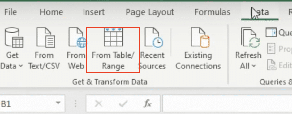
- If your data isn’t in a table format, Excel will prompt you to create one.
Step 2: Select columns for grouping duplicates.
- In the Power Query Editor, identify the columns you want to use as the basis for grouping duplicates.
- These are typically columns with unique identifiers or categories.
Step 3: Use the Group By feature.
- Click on “Group By” in the “Home” tab of Power Query Editor.

- In the Group By dialog box, select the column(s) you want to group by.
Step 4: Choose aggregation methods.
- For each additional column, select how you want to aggregate the data.
- Options include Sum, Average, Count, Max, Min, and more.
- You can add multiple aggregations for each column if needed.
Step 5: Apply changes and load results.
- Click “OK” to apply the grouping and aggregations.
- Review the results in the Power Query Editor.
- If satisfied, click “Close & Load” to send the data back to your Excel worksheet.

Power Query offers more flexibility and power in handling large datasets and complex grouping scenarios compared to traditional Excel functions.
How to Group All Duplicates Together in Excel
Grouping duplicates visually can help in data analysis. Here’s how to do it:
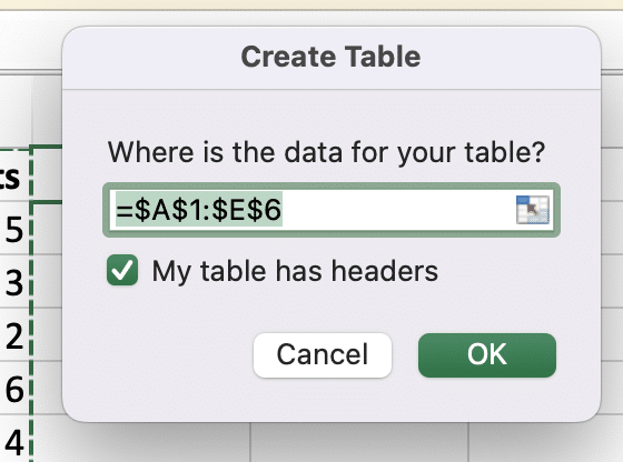
Step 1: Create a Table.
- Select your data range.
- Press Ctrl + T or click “Format as Table” in the “Home” tab.
- Ensure “My table has headers” is checked if applicable.
Step 2: Add a helper column.
- In the first empty column of your table, enter this formula: =COUNTIF($A$2:$A2,$A2)

- Adjust the column reference (A) to match your data.
- This formula counts occurrences of each value, assigning numbers to duplicates.
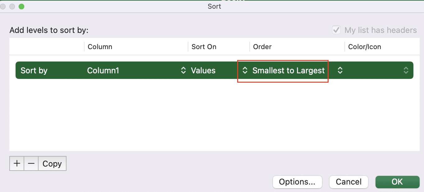
Step 3: Sort your data.
- Select any cell in your table.
- Go to the “Data” tab and click “Sort.“

- Sort by your helper column in ascending order, then by your original data column.
Step 4: Use Conditional Formatting.
- Select your data range.
- Go to “Home” > “Conditional Formatting” > “New Rule“.

- Choose “Use a formula to determine which cells to format“.
- Enter this formula: =$HelperColumn2<>$HelperColumn1
- Replace HelperColumn with your actual column letter.
- Choose a format to highlight changes between groups.
Step 5: Apply Excel’s Subtotal feature (optional).
- With your sorted data selected, go to “Data” > “Subtotal“.

- Choose the column to group by, the function to use (e.g., Count), and which value columns to subtotal.
- Click OK to add subtotals and outline groups.
This method visually groups duplicates and provides a structure for further analysis.
Combining Matching Data from Multiple Sheets
When you have matching data spread across multiple sheets, you can combine them using Excel’s Consolidate feature:
Step 1: Ensure consistent column headers.
- Review all sheets you want to combine.
- Make sure column headers are identical and in the same order on each sheet.
Step 2: Use the Consolidate feature.
- Go to a new sheet where you want the combined data.
- Click on the “Data” tab in the ribbon.
- Select “Consolidate” in the “Data Tools” group.

Step 3: Set up the consolidation.
- In the Function drop-down, select “Sum” (even for text data, this will combine entries).
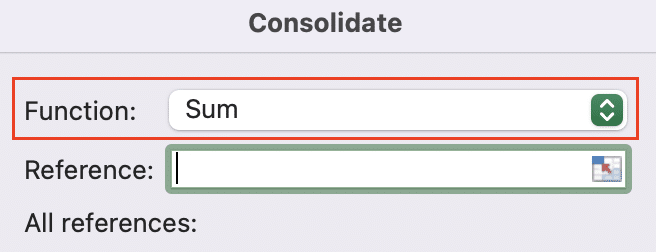
- Click in the Reference box, then select the entire data range from your first sheet.
- Click “Add” to include this range.
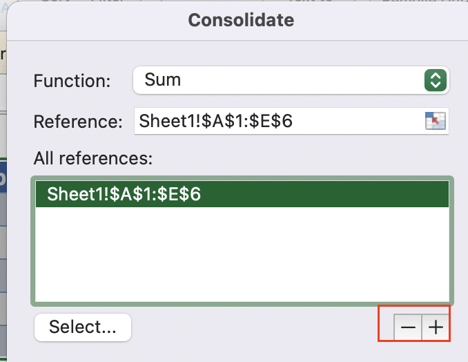
- Repeat for each sheet you want to combine.
Step 4: Configure labels.
- Check the boxes for “Top row” and “Left column“.
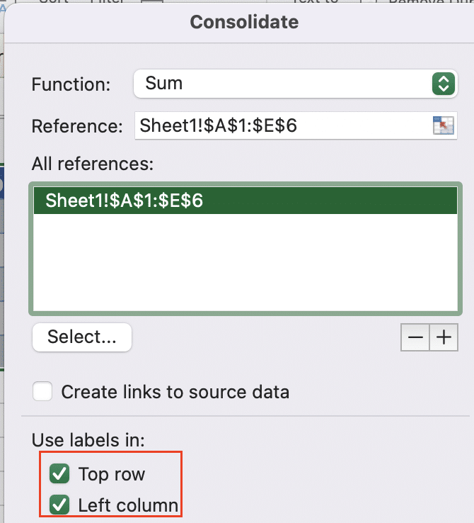
- This tells Excel to use your column and row headers.
Step 5: Finalize and review.
- Click “OK” to consolidate your data.
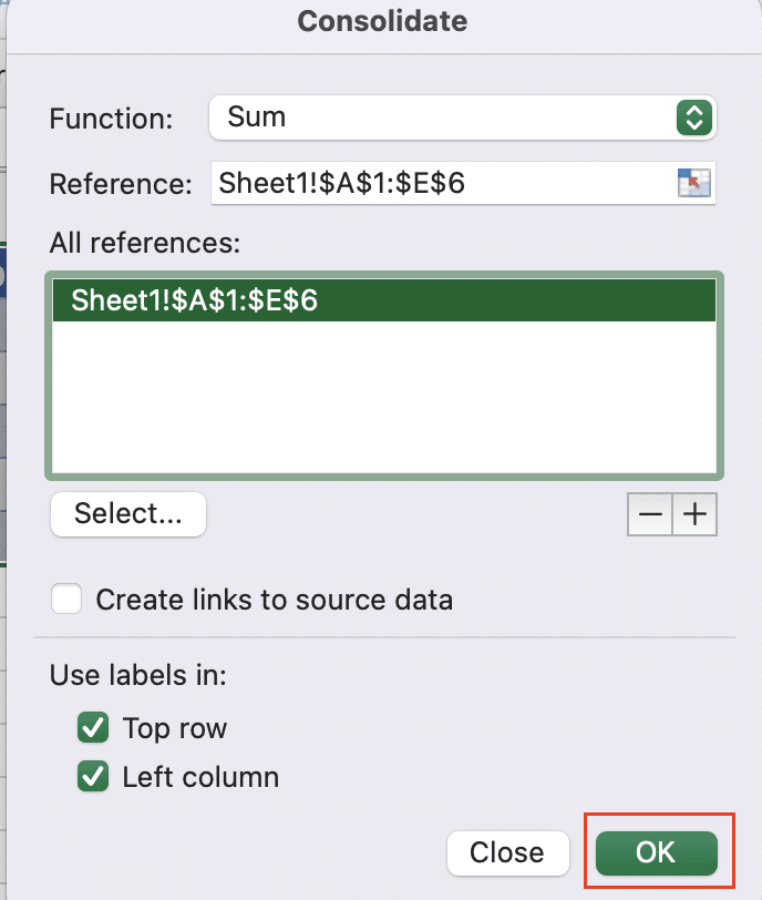
- Excel will combine matching data from all selected sheets.
- Review the consolidated data for accuracy.
- Format the resulting table as needed.
This method is particularly useful when you have consistent data structures across multiple sheets or workbooks.

Stop exporting data manually. Sync data from your business systems into Google Sheets or Excel with Coefficient and set it on a refresh schedule.
Get Started
Automating Duplicate Combination with VBA
For repetitive tasks involving duplicate combination, VBA (Visual Basic for Applications) can automate the process:
Step 1: Open the Visual Basic Editor.
- Press Alt + F11 in Excel to open the VBA editor.

- If you don’t see the Project Explorer, press Ctrl + R.
Step 2: Insert a new module.
- Right-click on your workbook name in the Project Explorer.
- Select Insert > Module.

Step 3: Paste the VBA code.
- In the new module, paste the following code:
vba
Copy
Sub CombineDuplicates()
Dim ws As Worksheet
Dim rng As Range
Dim lastRow As Long
Set ws = ActiveSheet
lastRow = ws.Cells(ws.Rows.Count, “A”).End(xlUp).Row
Set rng = ws.Range(“A1:C” & lastRow)
rng.RemoveDuplicates Columns:=Array(1), Header:=xlYes
ws.Range(“D1”).Value = “Combined Text”
ws.Range(“E1”).Value = “Sum of Values”
ws.Range(“D2”).Formula = “=TEXTJOIN(“”, “”, FILTER(OriginalData!C$2:C$” & lastRow & “, OriginalData!A$2:A$” & lastRow & “=A2))”
ws.Range(“E2”).Formula = “=SUMIF(OriginalData!A$2:A$” & lastRow & “, A2, OriginalData!B$2:B$” & lastRow & “)”
ws.Range(“D2:E2”).AutoFill Destination:=ws.Range(“D2:E” & lastRow)
End Sub
Step 4: Customize the code.
- Adjust column references (A, B, C) to match your data structure.
- Modify the “OriginalData” sheet name if different.
Step 5: Create a button to run the macro.
- Go back to your Excel sheet.
- Click “Developer” > “Insert” > “Button” (Form Control).

- Draw a button on your sheet.
- Assign the “CombineDuplicates” macro to this button.
Step 6: Test the automation.
- Make a copy of your data for testing.
- Click the button to run the macro.
- Review the results to ensure it’s working as expected.
This VBA solution offers a quick way to combine duplicates with a single click, saving time on repetitive tasks.
Streamline Your Excel Workflow
By mastering these techniques for combining duplicates in Excel, you’ll significantly enhance your data management efficiency. Start implementing these methods today to streamline your spreadsheet workflows and improve data clarity.
Ready to take your data management to the next level? Get started with Coefficient for even more powerful data solutions that seamlessly integrate with your existing spreadsheets.

