Want to supercharge your spreadsheets with clickable links that update automatically? Combining the power of VLOOKUP and HYPERLINK functions lets you create dynamic reference systems that work seamlessly in both Excel 2025 and Google Sheets. In this step-by-step tutorial, we’ll walk through exactly how to set up these formulas to build efficient cross-sheet navigation.
Create Your First VLOOKUP Hyperlink
To get started, set up your source data in columns, with the target URLs in one column and the display text you want to show for each link in another. Then enter the basic HYPERLINK(VLOOKUP()) formula structure in a new cell and test out the link functionality.
Build the Basic Formula
The key is to first write the VLOOKUP portion of the formula to find your target URL based on a lookup value. Then wrap the entire VLOOKUP in a HYPERLINK function. Finally, add your display text as the second parameter in the HYPERLINK.
For example:
=HYPERLINK(VLOOKUP(lookup_value, table_array, col_index_num, FALSE), display_text)

Add Reference Tables
To make your VLOOKUP work, structure your data as a lookup table, with the URLs you want to link to in one column and user-friendly display names in another. Keeping this table well-organized will make your formulas more efficient.
Link Across Different Sheets
What if the URL you want to link to is on a different worksheet? No problem. You can easily create references to cells on other sheets within your VLOOKUP. Just use absolute cell references for stability and be sure to handle any spaces or special characters in your sheet names.
Cross-Sheet Formula Examples
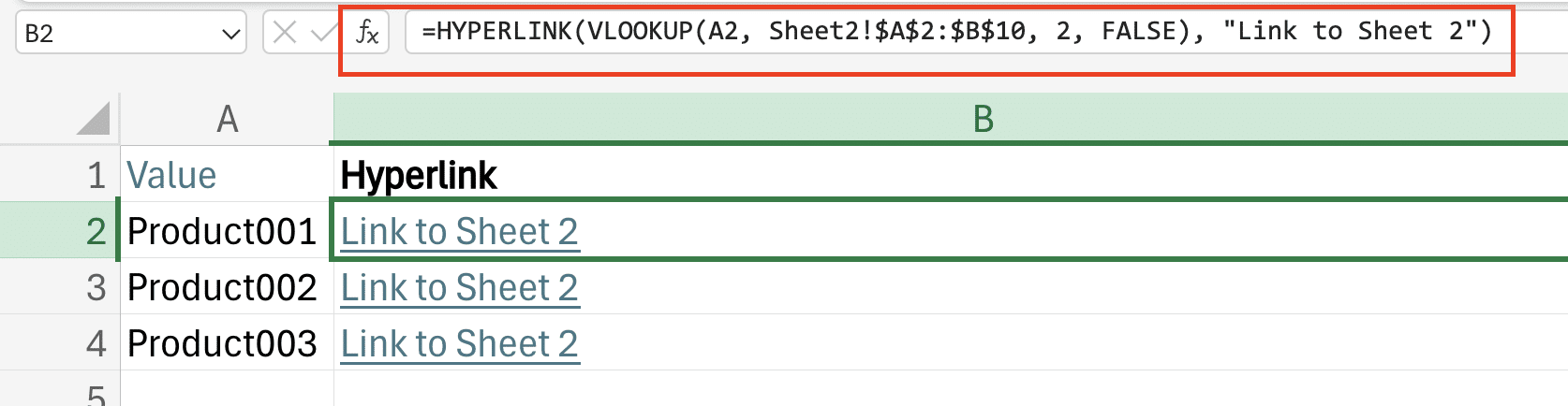
Here’s how you could link to a specific cell on another worksheet:
=HYPERLINK(VLOOKUP(A1,’Sheet 2′!$A$2:$B$10,2,FALSE), “Link to Sheet 2”)
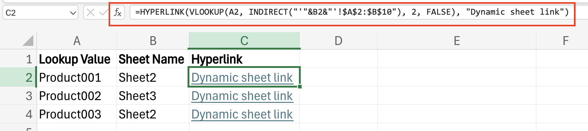
To create dynamic sheet references, you can use the INDIRECT function:

Stop exporting data manually. Sync data from your business systems into Google Sheets or Excel with Coefficient and set it on a refresh schedule.
Get Started
=HYPERLINK(VLOOKUP(A1,INDIRECT(“‘”&B1&”‘!$A$2:$B$10”),2,FALSE), “Dynamic sheet link”)
Customize Your Hyperlinks
Once you have the basic VLOOKUP hyperlink set up, you can customize the appearance and behavior of your links. Use cell formatting to change the color and style. Add hover text with the HYPERLINK function’s info_text parameter for a better user experience. You can even set up conditional formatting rules to change the link appearance based on certain criteria.
Formula Variations for Different Needs
There are a few ways you can tweak the VLOOKUP hyperlink formula depending on your specific needs:
- Use relative cell references if you want to the formula and have it update for each row
- To create many hyperlinks at once, use an array formula (entered with Ctrl+Shift+Enter)
- If your URLs or display text will update frequently, reference those cells dynamically in your formulas
Next Steps
Ready to put this into practice? Start by applying these VLOOKUP hyperlink techniques to your own spreadsheets. Set up some sample lookup tables and experiment with different formulas. Before long, you’ll be creating sophisticated navigation systems that make your spreadsheet data more accessible than ever.
Looking for an even easier way to build dynamic dashboards with your spreadsheet data? Check out Coefficient to sync live data into Excel and Google Sheets and create interactive reports with just a few clicks.


