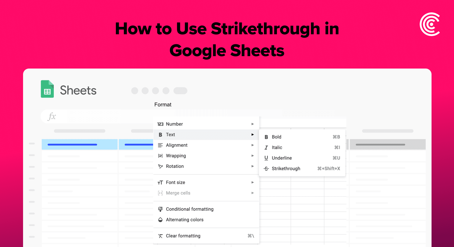
TL;DR: Apply strikethrough in Google Sheets by selecting text or cells and using ‘Format’ > ‘Text’ > ‘Strikethrough’ or Alt + Shift + 5 (Cmd + Shift + X on Mac). Remove it using the same steps.
This guide will show you how to apply and remove strikethrough in your Google Sheets.
Step 1: Open Your Google Sheet
Start by opening the Google Sheets document where you want to apply strikethrough.
Step 2: Select the Text or Cell
Click on the cell that contains the text you want to strike through. If you want to strikethrough only part of the text in a cell, double-click the cell and highlight the specific text.
Step 3: Applying Strikethrough

Supercharge your spreadsheets with GPT-powered AI tools for building formulas, charts, pivots, SQL and more. Simple prompts for automatic generation.

With the text or cell selected, click on the ‘Format’ menu in the menu bar. Hover over ‘Text’ and then click on ‘Strikethrough.’ You can also use the keyboard shortcut Alt + Shift + 5 (Cmd + Shift + X on Mac).
Step 4: Removing Strikethrough
To remove strikethrough, simply select the cell or text again and repeat the same process: ‘Format’ > ‘Text’ > ‘Strikethrough’, or use the keyboard shortcut.
Tips for Using Strikethrough Effectively:
- Task Management: Use strikethrough for task lists in your sheet to visually indicate completed items.
- Data Correction: Highlight corrections in data sets by using strikethrough on the original text and adding the corrected data nearby.
- Visual Consistency: Keep your sheet visually organized by using strikethrough consistently across similar types of data or tasks.


