Creating a bar graph in Google Sheets is an effective way to visually compare data across categories or groups. Whether it’s sales data, revenue growth, or customer demographics, bar graphs made in Google Sheets are customizable and visually appealing.
This guide will take you through the process of creating a bar graph, from data selection to chart customization.
Understanding Bar Graphs
Bar graphs are a versatile and effective way of visually representing data. They employ rectangular bars of varying lengths or heights to display information, with each bar representing a specific category or group. The length or height of these bars signifies the values or frequencies of the data points being presented.
One of the primary advantages of using bar graphs is their ability to reveal patterns, trends, and comparisons among the data. Comparing different categories becomes much more straightforward since the bars allow for a side-by-side representation, making data interpretation more accessible and faster for the reader.
There are several types of bar graphs, such as horizontal and vertical graphs, each with its unique applications:
- Vertical bar graphs are more commonly used as they make it easier to compare values across categories.
- Horizontal bar graphs are better suited for visualizing data with lengthy labels or numerous groups, as they offer more space for label presentation.
Accessing and Setting Up Google Sheets
Google Sheets is a powerful online spreadsheet application that allows users to create, edit, and share various types of data in a tabular format.
To begin working with Google Sheets, you’ll need to create a new sheet. Here’s how:
- Open Google Drive and sign in.
- Click ‘+New’ and select ‘Google Sheets’ from the dropdown.
Alternatively, type sheets.new in your browser’s address bar and press Enter.
Now, let’s walkthrough how to make a bar graph in Google Sheets.
Step-by-Step Guide: How to Make a Bar Graph in Google Sheets
Step 1: Input Your Data
First, open a new Google Sheets document. In our example, we’re going to create a graph representing monthly sales figures over a six-month period. The data is structured with ‘Month’ as one category and ‘Sales ($)’ as another.
| Month | Sales ($) |
| January | 1200 |
| February | 1500 |
| March | 1800 |
| April | 1350 |
| May | 1600 |
| June | 2000 |
Step 2: Select the Data You want to Graph
Once your data is in place, it’s time to select what you want to include in your graph. This selection is known as the ‘data range’.
Click and drag your mouse over the cells containing your data, including the column headings. For our sample data, you’ll select from A1 to B7.
The selection you make here depends on the data you want to visualize. In our case, we’re including both the months and their corresponding sales figures. Including the headers in your selection ensures that Google Sheets correctly labels the axes of your graph.
Step 3: Choose the Appropriate Graph Type
Now, click on the ‘Insert’ menu at the top of your screen, then choose ‘Chart’.
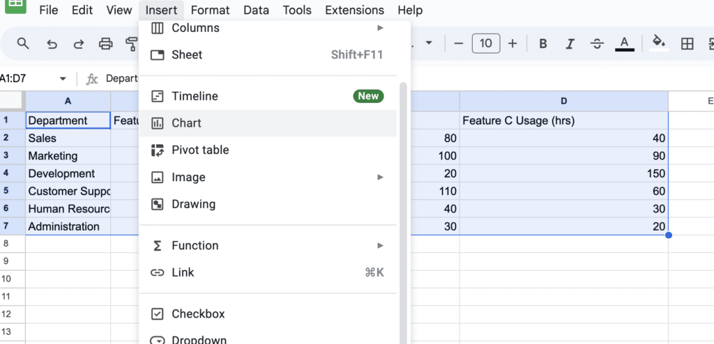
Google Sheets will automatically suggest a chart type. For sales data over time, a bar chart is typically most effective.
If the suggested chart isn’t a bar chart, or if you prefer a different style, use the Chart Editor on the right side of the screen. Here, you can change the chart type and see the effect on your data in real-time.

Supercharge your spreadsheets with GPT-powered AI tools for building formulas, charts, pivots, SQL and more. Simple prompts for automatic generation.

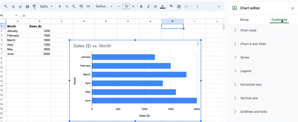
Step 4: Customize Your Graph
With your chart inserted, it’s time to customize. The Chart Editor offers various options to modify your graph.
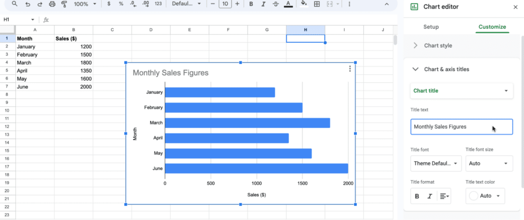
You can change the title to something more descriptive like “Monthly Sales Figures.”
Navigate to the Chart editor and select the ‘Customize’ tab.
Click the ‘Chart & axis titles drop-down.’
Enter “Monthly Sales Figures” under ‘Title text.’
Your bar chart title will change automatically.
Customize other elements like the bar colors, axis labels, and legend for clarity and visual appeal. For example, you might want to use different colors for each month or adjust the scale of the sales figures for better readability.
Conclusion
Creating a bar graph in Google Sheets is straightforward and allows for significant customization to suit your specific needs. To further enhance your data analysis capabilities in Google Sheets, consider installing Coefficient.
Coefficient offers advanced data integration and analytics features, making it an invaluable addition for anyone looking to derive deeper insights from their data. Install it for free and try it with your business data today!


