How to Hide Rows in Google Sheets: A Step-by-Step Guide

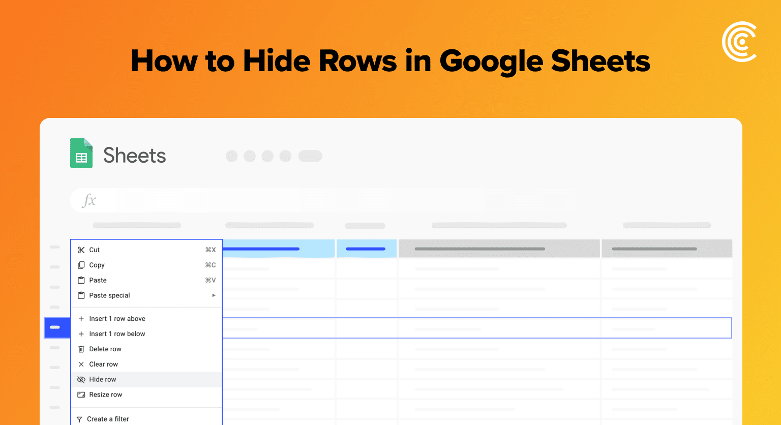
To hide a row in Google Sheets, simply select the row or rows you want to hide by clicking on the row number(s) on the left-hand side of the spreadsheet. Once the row(s) are selected, right-click and choose “Hide row” from the context menu. Alternatively, you can use the keyboard shortcut Shift+9 to hide the selected row(s).

Step-by-Step Guide to Hiding Rows

Hiding rows in Google Sheets is a simple and useful feature that can help you organize your data and make your spreadsheets look cleaner. In this section, we will provide a step-by-step guide to hiding rows in Google Sheets.

Hiding Single Rows

To hide a single row in Google Sheets, follow these steps:

1. Select the row you want to hide by clicking on the row number on the left-hand side of the screen.
2. Right-click on the row number and select “Hide row” from the drop-down menu. Alternatively, you can use the keyboard shortcut “Ctrl + Alt + 9” to hide the selected row.

Once you have hidden a row, it will disappear from view, but the row number will remain visible. To unhide a row, simply select the rows above and below the hidden row, right-click, and select “Unhide rows” from the drop-down menu.

Hiding Multiple Rows

If you want to hide multiple rows at once in Google Sheets, follow these steps:

1. Select the rows you want to hide by clicking and dragging your mouse over the row numbers on the left-hand side of the screen. Alternatively, you can hold down the “Shift” key and click on the first and last row you want to hide to select all the rows in between.
2. Right-click on any of the selected row numbers and select “Hide rows” from the drop-down menu. Alternatively, you can use the keyboard shortcut “Ctrl + Alt + 9” to hide the selected rows.

Once you have hidden multiple rows, they will disappear from view, but the row numbers will remain visible. To unhide multiple rows, simply select the rows above and below the hidden rows, right-click, and select “Unhide rows” from the drop-down menu.

In conclusion, hiding rows in Google Sheets is an easy way to organize your data and make your spreadsheets look cleaner. By following the simple steps outlined in this section, you can quickly and easily hide single or multiple rows in Google Sheets.

W

Selecting Non-Continuous Rows

To select continuous rows in Google Sheets, you can use the following steps:

1. Click on the first row you want to select.
2. Hold down the Ctrl key (Windows) or Command key (Mac) on your keyboard.
3. Click on the next row you want to select.
4. Repeat steps 2-3 for all the rows you want to select.

Alternatively, you can use the following steps to select non-continuous rows in Google Sheets:

1. Click on the first row you want to select.
2. Hold down the Shift key on your keyboard.
3. Click on the last row you want to select.
4. Hold down the Ctrl key (Windows) or Command key (Mac) on your keyboard.
5. Click on the next row you want to select.
6. Repeat steps 4-5 for all the rows you want to select.

Hiding Non-Continuous Rows

Once you have selected the non-continuous rows you want to hide, you can use the following steps to hide them:

1. Right-click on one of the selected rows.
2. Click on the “Hide rows X-Y” option in the context menu that appears, where X and Y are the first and last rows in the selection.

Alternatively, you can use the following steps to hide non-continuous rows in Google Sheets:

1. Click on the “Format” menu at the top of the screen.
2. Click on “Hide rows” in the drop-down menu.
3. Enter the row numbers you want to hide in the dialog box that appears, separated by commas.

It is important to note that hiding non-continuous rows in Google Sheets does not delete the data in those rows. The data is simply hidden from view, but it can be unhidden at any time. To unhide non-continuous rows, simply select the rows before and after the hidden rows, right-click on them, and click on “Unhide rows” in the context menu that appears.

In conclusion, hiding non-continuous rows in Google Sheets is a simple process that can be accomplished using the steps outlined above. By following these steps, you can easily hide and unhide non-continuous rows in your Google Sheets document.

Unhiding Rows for Data Review

Sometimes, you may need to unhide rows in Google Sheets to review data that was previously hidden. Fortunately, unhiding rows in Google Sheets is just as easy as hiding them. In this section, we will cover how to unhide single and multiple rows in Google Sheets.

Unhide Single Row

To unhide a single row in Google Sheets, follow these steps:

1. Right-click on the row number above and below the hidden row. For example, if row 5 is hidden, right-click on row 4 and row 6.
2. Select “Unhide row X” from the context menu, where X is the number of the hidden row. Alternatively, you can click on “Unhide row X” from the “Rows” menu at the top of the screen.

Unhide Multiple Rows

To unhide multiple rows in Google Sheets, follow these steps:

Free AI-Powered Tools Right Within Your Spreadsheet

Supercharge your spreadsheets with GPT-powered AI tools for building formulas, charts, pivots, SQL and more. Simple prompts for automatic generation.

1. Select the rows above and below the hidden rows. For example, if rows 5 to 7 are hidden, select rows 4 and 8.
2. Right-click on the selected rows and choose “Unhide rows” from the context menu. Alternatively, you can click on “Unhide rows” from the “Rows” menu at the top of the screen.

It’s important to note that when you unhide rows in Google Sheets, they will be unhidden in the same order that they were hidden. For example, if you hide rows 5, 6, and 7 in that order, and then unhide them, they will be unhidden in the same order: 5, 6, and 7.

In conclusion, unhiding rows in Google Sheets is a simple process that can be done in just a few clicks. Whether you’re reviewing data or making changes to your spreadsheet, unhiding rows is an essential skill that every Google Sheets user should know.

Managing Rows on Mobile Devices

Managing rows on mobile devices can be a bit different than on desktop. However, it is still possible to hide rows on Google Sheets using your iOS or Android device.

Hiding Rows on iOS

To hide rows on iOS, you need to follow these steps:

1. Select the row(s) you want to hide by tapping on the row number(s) on the left side of the screen.
2. Tap on the three dots in the top right corner of the screen.
3. Tap on “Hide Row” from the menu that appears.

The hidden rows will be marked with a thicker line, indicating that they are hidden. To unhide the rows, simply follow the same steps and tap on “Unhide Row” instead.

Hiding Rows on Android

To hide rows on Android, you need to follow these steps:

1. Select the row(s) you want to hide by tapping on the row number(s) on the left side of the screen.
2. Tap on the three dots in the top right corner of the screen.
3. Tap on “Hide Row” from the menu that appears.

The hidden rows will be marked with a thicker line, indicating that they are hidden. To unhide the rows, simply follow the same steps and tap on “Unhide Row” instead.

It is important to note that hiding rows on mobile devices may not be as precise as on desktop. This is because the screen size is smaller, and it can be harder to select the exact row(s) you want to hide. However, with a bit of practice, you should be able to hide rows on your mobile device with ease.

Overall, hiding rows on mobile devices is a straightforward process. Whether you are using an iOS or Android device, you can easily hide rows on Google Sheets using the steps outlined above.